If groundwater levels must be interpolated, a simple interpolation of the measured values does not usually provide a satisfactory result. In fact, the model files often already contain information that should be taken into account during interpolation. This includes:
Fixed potentials heads(POTE),
Source/sink terms (KNOT),
Receiving water course (VORF and LERA or LEKN as idealised leakage data ),
Areas with the same unknown potential heads (GLEI),
Minimum values for the distance between the surface and groundwater level,
No-flow boundary conditions and
Transmissivities (TRAN)
The individual data is defined in the following menu window. Which is accessed by activating the "Additional interpolation points" checkbox.
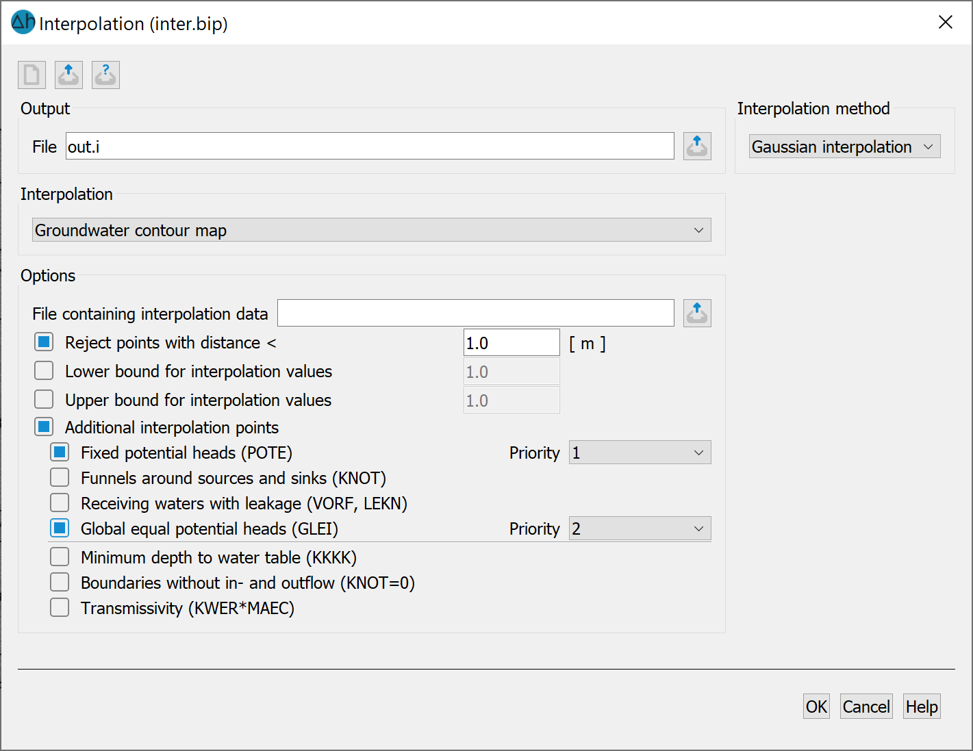
Inputs for the interpolation of a groundwater contour map
After each interpolation run, one or more potential head values are generated as additional interpolation points for a new interpolation in the respective local effective range of the listed influencing variables. The results from an initial interpolation of the measured values (file with interpolation data) to the FE nodes are used as base values for determining these interpolation points.
Only the menu items for which the corresponding attribute already exists in the model file appear as "Additional interpolation points".
Example:
If only the LERA attribute is assigned in the model file instead of the LEKN attribute, the "receiving waters with leakage" checkbox item will not be available (LEKN must be explicitly assigned!).
(1) Fixed potential heads: The nodes assigned with POTE are used like measured values as additional interpolation points for a new interpolation.
(2) funnels around sources and sinks: For all nodes assigned the KNOT attribute, support points are generated for all nodes within the estimated range and assigned the lowered (or increased) potential heads for a new interpolation. For this purpose, data for K-values (KWER) and element thicknesses of the aquifer must be available for the entire area after a model check has been carried out. The thicknesses do not necessarily have to be defined using the MAEC data type, but can also result from the calculation of the initial and maximum thicknesses.
(3) Receiving waters with leakage:
For nodes with defined reference water level for watercourses, the qualitative influence of a watercourse on the groundwater can be simulated by defining a substitute leakage coefficient. For this purpose, values between 0 (no groundwater contact) and 1 (complete groundwater contact) must be defined at nodes with defined reference water level for watercourses using the LEKN attribute. Additional support points are then generated at these nodes. The calculation of the potential head is linear between the reference water level for watercourses and the interpolated potential heads.
Attention: Consideration of this influencing variable may require the replacement of the leakage coefficient LERA required for the model calculation. Calculations other than the interpolation of groundwater contour maps with the replacement coefficients used here can lead to serious errors! Therefore, restore the original values after completing the interpolation or delete the LEKN replacement values from the mesh file using the editor or via the Attributes  → Delete... menu item
(4) Areas with equal potential heads: The procedure for considering GLEI areas corresponds to the procedure for interpolating node data. The potential heads of the GLEI nodes are replaced by an averaged value. In contrast to the consideration of GLEI areas in the interpolation of node data, the spatial effect of these areas is taken into account in the subsequent interpolation.
(5) Minimum distance between surface and groundwater level: The KKKK attribute (general node data) can be used to check node potential heads for compliance with a minimum distance between the surface elevation and groundwater elevation. For this purpose, a minimum distance greater than 0 must be specified at the corresponding nodes. These values are then checked for compliance before and after each interpolation run.
(6) Boundaries without in- and out flow: To take no-flow boundary conditions into account, the affected boundary sections can be labelled with the KNOT attribute and the value 0. Constraint points are then generated on both sides of the resulting boundary polylines by mirroring the boundary element centres. The potential heads at these points are determined with the help of an additional interpolation with a maximum of 5 iteration steps if necessary..
(7) Transmissivity: The effect of the hydraulic conductivity (KWER) and the initial thickness (MAEC) can be taken into account by determining the element transmissivities between 2 measuring points in each section. Additional sampling points are only generated in areas without sampling points from other influencing variables and only if the transmissivity between two measuring points changes by at least 10%.
Priorities:
When considering these influencing variables (1)-(4), the situation may arise that different influences generate support points on the same FE node. As this can lead to local contradictions, a clear, complete priority must be specified to take these special cases into account. The number 1 corresponds to the highest priority.
The priority is assigned in the order in which the influencing variables are selected, but can also be edited subsequently. It is not necessary to assign priorities for the other influencing variables, as the interpolation points are based on the values determined up to that point. The processing sequence of the influencing variables (5)-(7) corresponds to their respective window position.
Interpolation with additional interpolation points generates the stuetzTMP.txt file in the format (I6, F10, F10, F10, without numbering), which contains all interpolation points created in addition to the measurement data file with the associated potential heads.
Stand: 30.01.2025 | 