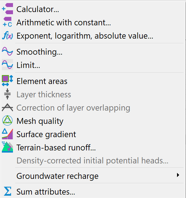
The following submenu appears:

 

 

Calculator…

The following window appears:

 

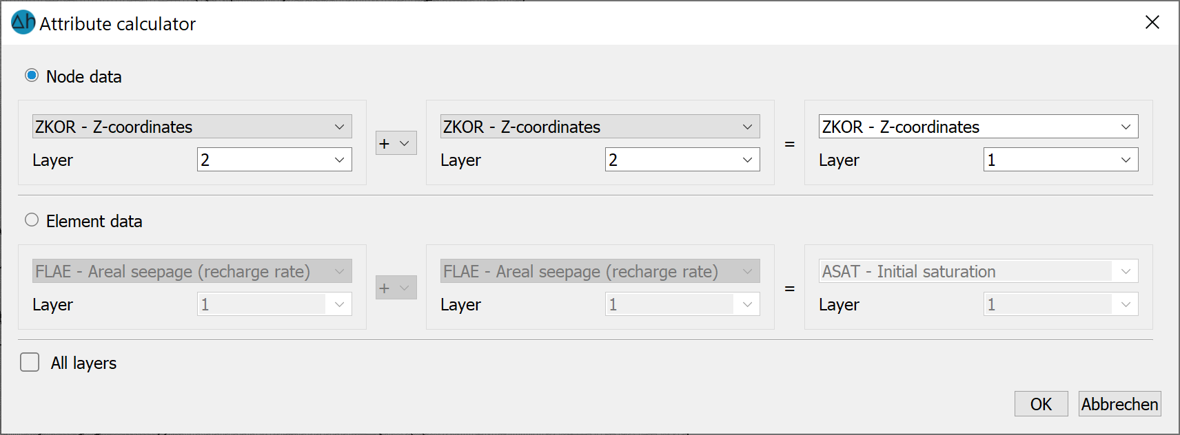
This menu item can be used to combine two node or two element data types into a third node or element data type.

In a 3D project, the data can only be processed in one layer or optionally in all layers.

The result identifier can be any identifier (also a new identifier unkown to SPRING). The data context determines whether SPRING saves this identifier as a node or element data type.

 

 

Arithmetic with constant…

The following window appears:

 

 

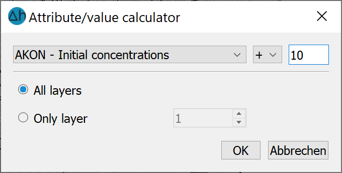
A selected node or element data type (for a 3D model in all or only one layer) can be calculated with a constant. The available calculation types are sum (+), subtract (-), multiply (*), divide (÷) and exponent (^). The selected identifier is offset against the constant and overwritten by the calculation result. There is no query as to whether the original values should really be overwritten by the calculation results or not. If the original values should be retained, then it is suggested to first copy the values to a new attribute identifier and performing the arithmetic operation upon that attribute.

 

 

Exponent, logarithm, absolute value…

In a 3D model the following window appears for a 3D model:

 

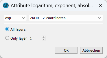
With a 2D model, there is no need to enter a node or element layer. With this menu item, existing attributes can be modified with the following functions:

f(x) = exp(x),

f(x) = 10^x,

f(x) = ln(x) or

f(x) = log(x)

f(x) = abs(x)

 

In a 3D model, the values of all layers or only the values of a single layer can be modified.

For each node or element (in all or only one layer) with a value x for the selected identifier, the existing value is converted using the selected function and overwritten by the calculation result f(x). There is no query as to whether the original values should really be overwritten by the calculation results or not.

 

 

Smoothing…

The following window appears for a 3D model:

 

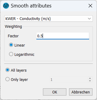
This menu item can be used to smooth node and element data by averaging the values.

The new value at a node/element is calculated from the old value and the average value of the surrounding nodes/elements:

 

Linear smoothing:

 

Logarithmic smoothing:

 

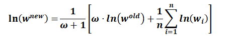
with:

w^neu:new value of a node or element

ω:weighting

w^alt:old value of the node or element

w_i:values of the surrounding nodes or elements

 

The larger the weighting factor ω is selected, the lower the smoothing.

For a 3D model, you can choose whether only the data of one layer or all layers should be smoothed. Only the element or node values horizontally neighbouring the element or node are used for smoothing, so that the attributes are only smoothed within their respective layer.

 

 

Limit…

The following window appears in a 3D model:

 

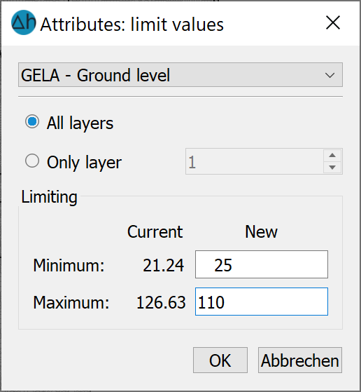
With this menu item, existing data can be limited upwards or downwards by defining limit values. For 3D models, the values of all layers or only the values of a single layer can be limited.

After selecting the desired identifier, the current minimum and maximum values of the attribute appear, which can be changed accordingly in the "New" field.

When the menu is closed with OK, all values found to be outside the new limit values are overwritten by the new minimum or maximum if they fall below or exceed them respectively.

 

 

Element areas

When this menu item is selected, the areas of all elements are calculated and saved under the AREA [m²] attribute

 

Layer thicknesses (3D model only)

The layer thicknesses in a 3D model is calculated by subtracting the Z-coordinates at the nodes as follows:

 

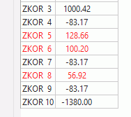
ZMAE (layer n) = ZKOR (layer n) - ZKOR (layer n+1).

 

The thicknesses for all layers are saved under the attribute ZMAE [m.

 

 

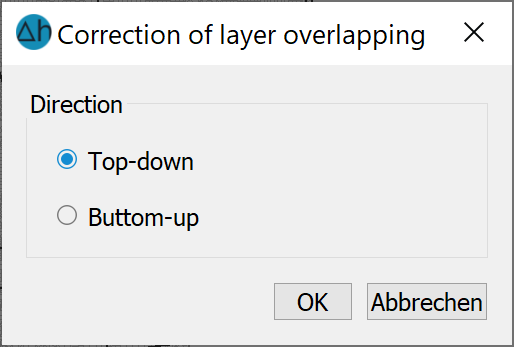
Correction of layer overlapping (3D model only)

If an object (e.g. a deep excavation) cuts into several layers, the nodes within the object must be placed on the lowest (or highest) affected element layer. This is done using this function.

 

The incorrect layer boundaries are coloured red in the node attribute dialogue:

 

Mesh quality

The quality of a finite element mesh and in particular the individual elements has a decisive influence on the results and the quality of the numerical calculations. Therefore, elements of poor quality should first be corrected after automatic mesh generation and before starting the calculations.

For the mesh quality, the deviation of any element from an ideal element is calculated, i.e. the deviation from an equilateral triangle or a quadrilateral. Two criteria are used in SPRING6, the Jacobi ratio and the shape factor.

The Jacobian ratio describes the deviation from ideal elements. For triangles, the Jacobian ratio is always 1 and for quadrilaterals it essentially describes the distortion of a rectangle. Mathematically, the Jacobian ratio is the ratio of the minimum determinant of the Jacobian matrix to the maximum determinant. This means that this ratio is always in the range between 0 and 1, with 1 corresponding to an ideal quadrilateral.

The shape factor is calculated from the ratio of the inner circle to the outer circle for all triangular elements. For quadrilateral elements, the ratio of the shortest side bisector to the longest distance between a corner point and the centre is used in the same way. For an ideal triangular element (equilateral triangle) this results in a value of 0.5, for a quadrilateral element a value of . For the mesh quality, these are rescaled so that the ideal element reaches the maximum of 1 in each case. Very small values indicate strongly degenerated elements.

The mesh quality rating is made up of the minimum of these two criteria. The mesh quality is saved under the attribute QLTY [-] in the model file

 

Surface gradient

The surface gradient is calculated for all elements and saved in the model file under the attribute GGRD [%].

 

 

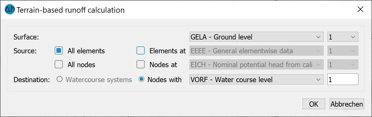
Terrain-based runoff

The following input dialogue appears:

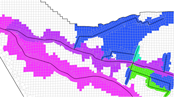
After performing this calculation, all elements whose surface runoff flows to a watercourse with a watercourse stage are assigned a runoff incidence value (attribute QE2V). This incidence value corresponds to the number of the model node to which the surface runoff of the corresponding element flows. An areal representation of the QE2V attribute illustrates the assignment (see figure).

 

Allocation of the terrain-based runoff

During the water system calculation, the discharge volume is assigned to the respective node by the VKNO attribute.

 

Density-corrected initial potentials

This menu item is only active if the AKON attribute is assigned in the model file (*.net or *.3d).

The potential head h [m] entered via EICH, POTE and VORF in the model files or the transient input file must be converted into pressures p for the density-dependent flow calculation:

 

p = (h - z) * ρ * g

 

This is done with the density ρ = ρ₀ for the concentration c₀ = 0 or the temperature T = T₀.

If the attributes 1KON or AKON are specified at nodes with potential heads and therefore the concentration c ≠ 0 (or T ≠ T₀ in the heat calculation), the potential heads must be calculated with the density ρ = ρ(c) and be converted into a "corrected" water level. This is done with the following dialogue:

 

 

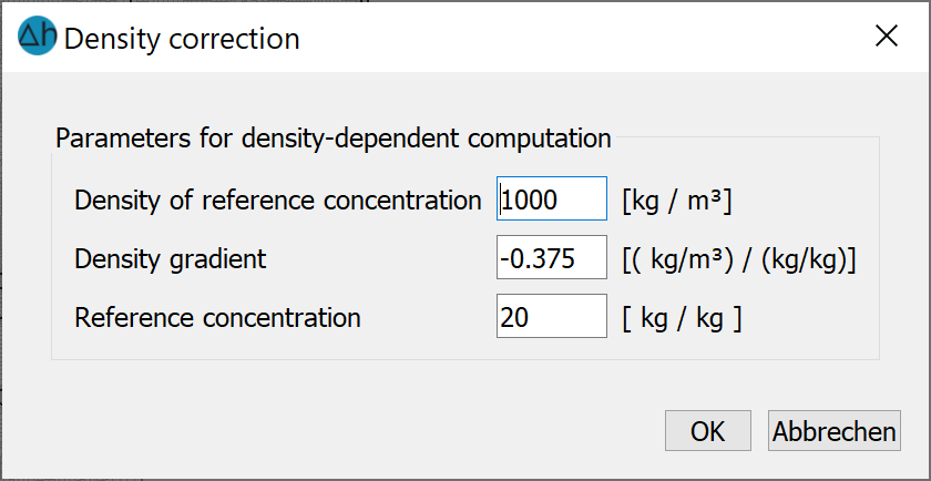
By entering the corresponding density parameters and confirming with OK, the potential heads are corrected and automatically saved in the model file. The parameters entered here correspond to the values entered in the density-dependent flow dialogue.

 

Example:

The formula for the density-corrected potential height h_korr is:

 

h_korr = (h_Start - z) * ρ/ρ₀ + z

with:

h_korr [m] = potential head corrected using the density parameters for POTE, EICH and VORF

h_Start [m] = POTE, EICH, or VORF at a node with specified 1KON or AKON

z [m] = height of the node, in the 3D model corresponds to the Z-coordinate, in vertical model with the Y-coordinate

ρ₀ [kg/m³] = density of the reference concentration at c₀ = 0

ρ [kg/m³] = known/desired density ρ(c = c_max), c_max is usually the maximum concentration entered as 1KON or AKON

 

The density gradient α required in the dialogue is obtained by converting the linear density function, which is implemented in the SITRA programme module:

 

ρ(c) = ρ₀ + α(c - c₀)

to:

α = (ρ(c_max) - ρ₀) / (c_max - c₀), if c = c_max is used.

 

Further information on the required parameters and conversions can be found in the chapter "Density-dependent mass transfer“ .

 

 

Groundwater recharge

There are four methods for determining groundwater recharge in SPRING:

 

• RUBINFLUX

This menu item leads to the transient groundwater recharge calculation with RUBINFLUX. A detailed description of the procedure and the input data can be found in the chapter: How To - "Calculation of a transient recharge rate" .

 

• According to Schroeder & Wyrwich with the following menu items:

 

 

• According to Meßer 2008 with the menu items:

 

• by soil water balance with the menu items:

 

If the basic attributes (KVNR, NATK or NCLC, NETP, FLUR, GELA) are available, the other attributes (NSFN, NMFN, NMKL, NMFK and NMGK) can be calculated at this point. The other parameters of the water balance equation (direct runoff NMAD and real evaporation NMET) can then be determined so that the recharge can be calculated last.

A detailed description of the procedures and the input data can be found in the chapter How To - "Calculation of mean recharge rates" and on the website:

"A simplified method for the calculation of area-differentiated groundwater recharge in Central Europe“.

 

 

Sum attributes…

The following window appears for a 3D model:

 

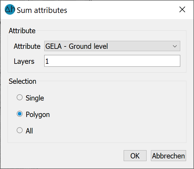
This menu item can be used to sum existing attributes individually, in a range or in total and, if necessary, for one or more layers. The result is then displayed in a dialogue.

 

Menu item: Copy attributes