The most important step for interpolation with the kriging method is therefore the creation of a variogram. This is used to relate the difference between two interpolation values to the distance between the corresponding interpolation points and to approximate the statistical information obtained in this way using a variance function:

In a first step, a so-called experimental variogram is created. Distance classes (distances in metres) are defined for this purpose:

 

For each distance class, the interpolation values of all pairs of interpolation points whose distances fall into this class are analysed and a semivariance g_k(h) is calculated:

 

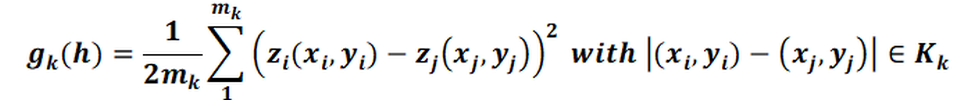
Where:

m_k denotes the number of all pairs of measuring points (i, j) whose distance is in the class K_k.

z_j denotes a point that is at a distance h from z_i.

A table with the most important variogram data of all distance classes is output for the subdivision of the distance classes selected by the user (maximum 16:

 

Column 1: number of class k,

Column 2: maximum distance h_k,

Column 3: mean distance h of all pairs of measuring points in this class, ,

Column 4: semivariance g_k(h)

Column 5: Number of all measuring point pairs in this class m_k,

Column 6 and 7: imax and jmax, numbers of the measuring points for which the interpolation values z(imax) and z(jmax) have the largest difference in the distance class,

Column 8: d(z(imax),z(jmax)) = 0.5 * (z(imax)-z(jmax))², as a comparison value for the variance g_k(h)

 

For example, such a table can look as follows for 10 distance classes with an equidistant subdivision for the classes:

 

Tabular output of the variogram parameters

 

The maximum distance between two interpolation values is also recorded for orientation purposes.

If possible, the distance classes should be categorised in such a way that the number of associated interpolation point pairs does not = 0 in any class. The number should be in the same order of magnitude for all distance classes. If a pair of interpolation points is not in any distance class, the maximum distance of the last class is increased accordingly.

In an experimental variogram, the calculated variances g_k(h) (column 4 of the table = y-axis) are now plotted against the mean distances h (column 3 of the table = x-axis) in a diagram. The boundary of the x-axis is the determined maximum distance between the interpolation points.

A function must now be found that approximates this experimental variogram as well as possible and can be used to calculate the interpolation weights λ_i(x, y).

Six function types are offered as starting functions for this:

• Variogram h^A

• Spherical variogram

• Exponential variogram

• Gaussian variogram

• Cubic polynomial

• Fitting polynomial

 

The parameters PEP, PI and A must be defined for types (1) to (5):

• PEP >= 0: so called 'nugget effect': A measure of the scattering of the interpolation values (interpolation error). g(0)=PEP.

• PI >= 0: Variance of the observed interpolation values.

• A >= 0: Size of the area whose points are used for interpolation, for function types (2) to (5) the parameter A should correspond approximately to the maximum distance.

 

The following diagram shows the meaning of the individual parameters:

 

Schematic representation of the variogram parameters

 

The following figures show the experimental variogram (red dots) overlaid with the selected function (blue) and the corresponding input in SPRING for the various approach functions.

 

(1) Variogram h^A:

The fitting function for this type of variogram is:

 

g(h) = PEP + PI * h^A

 

Depending on the parameter A, there are three different function curves of the variogram:

 

Case 1: A = 1 (straight line)

 

 

Case 2: A < 1

 

 

Case 3: A > 1

 

 

 

(2) Spherical variogram:

The approach function for this type of variogram is:

 

 

 

 

 

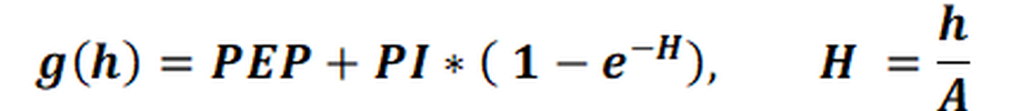
(3) Exponential variogram:

The approach function for this type of variogram is:

 

 

 

(4) Gaussian variogram:

The approach function for this type of variogram is:

g(h) = PEP + PI *( 1-exp (-H²)), with H = h/A

 

 

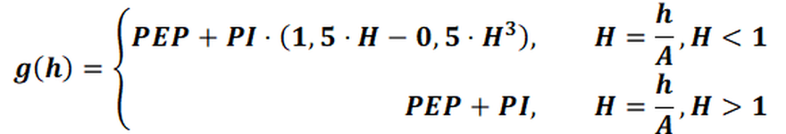
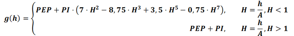
(5) Cubic polynomial:

The approach function for this type of variogram is:

 

 

 

(6) Fitting polynomial of a degree between 1 and 9

If a fitting polynomial is selected, the degree of the polynomial (between 1 and 9) and the number of points for which the polynomial is to be approximated (maximum number is the number of distance classes) must be specified.

The experimental variogram, for example, results in the following fitting polynomial:

 

 

In general, the appropriately constructed functions should be monotonically increasing and approximate the calculated values as well as possible. The quality of the variance function g(h) ultimately determines the quality of the points interpolated with Kriging.

When using the kriging interpolation method, particular importance must be attached to the creation of the variogram, as the interpolation method reacts particularly sensitively to the choice of parameters.

 

Kriging Interpolation