Structure data from "non-project" files (external format) can also be imported into an existing project. These files do not have to be in *.str format. Via the Structure → Import… menu item a number of different formats can be imported, including: *.str, *.txt, *.csv, *.arc, and *.shp.

In this example, the structure data file "s3_Daten2.str" is included. It is available for download on our website (directory: .../Tutorial_bsp_files/Tutorial_2D_bsp_files/...).

The new included structures are: Depth information of the model as UNTE, a MARKing of the stream course and the line-wise leakage value of the stream course (LERA). While the MARK and LERA attributes can be assigned directly, as described in the chapter "Direct assignment of existing structural data", the UNTE attribute (model lower boundary) must be interpolated element by element in this example.

The inputs for the individual interpolation methods are described in detail in the chapter "Calculation - Interpolation".

By opening the Attributes Assign By interpolation... menu item, the following windows appears:

Interpolation of element data

 

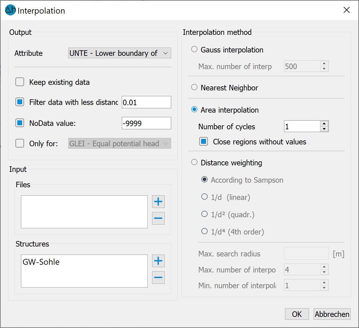
Select the input: Add from structures (), a further selection menu opens in which all existing structure data is listed. Select the structure with the "UNTE" data type. UNTE" is also selected as the output attribute data type:

 

Note: The output data type can differ from the identifier of the structure data type selected for interpolation!

Area interpolation is selected as the interpolation method. After pressing the OK button, the data is interpolated and the following control window appears after successful calculation:

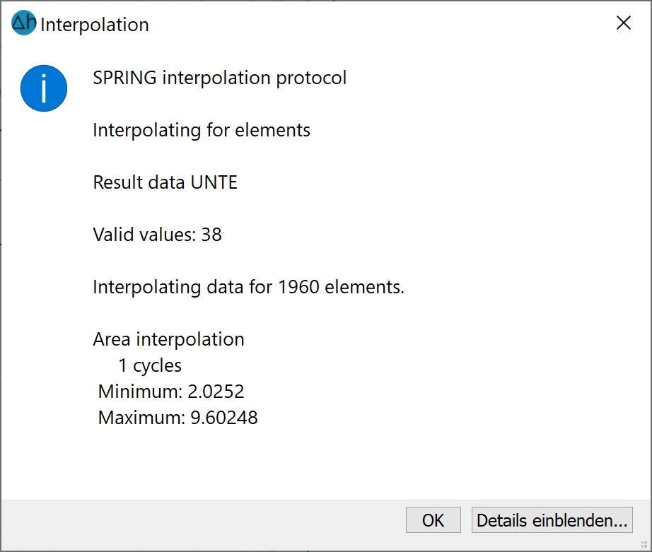
Interpolation protocol

 

The next step is to interpolate the initial potential head values. This must be carried out with particular care, as the initial potential heads are one of the most important types of data for calibrating the groundwater model. As a rule, groundwater measuring points that were obtained from the study area are required for calibration and should be used as the basis for the initial potential heads. In addition, information on the water levels of the main receiving stream (POTE) and the tributary (VORF) must be known. An initial potential head state is determined from these three types of data by interpolation, which must then be manually revised after an initial visualisation.

An example of a necessary revision are interpolated groundwater comparisons that show infiltration into the groundwater where there is none. This situation was created by the bed elevation of small tributary waters that was used as the receiving water elevations, however, these tributaries do not carry any water at all. In this case, the receiving water heights at such nodes must be deleted for the interpolation.

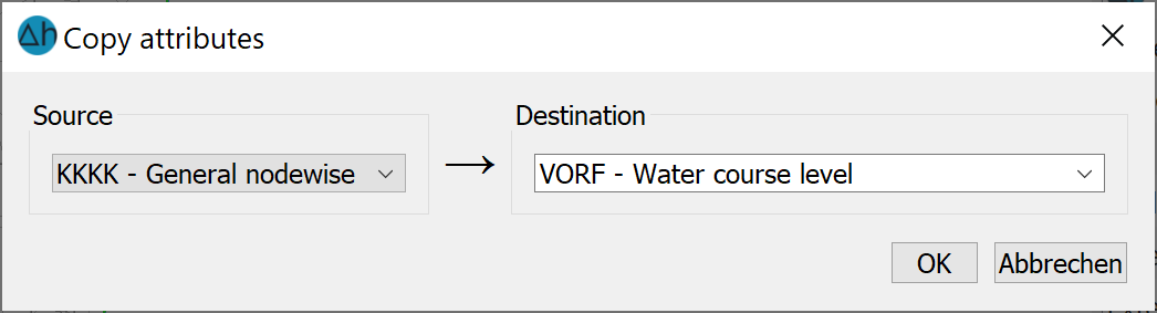
To take the VORF and POTE attributes into account (which has already been assigned in the chapter "Direct assignment of existing structural data"), "VORF" and "POTE" must first be transferred via Attributes Copy Attribute-wise... to "EICH" to be included in the interpolation as "existing data".

 

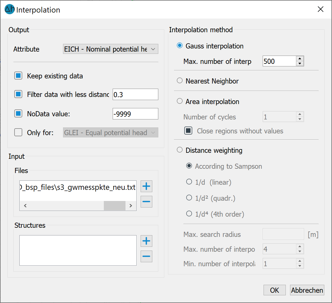
Via Attributes Assign By interpolation... the window for interpolating node data appears. There, under Input: Files, the file "s3_gwmesspkte_neu.txt" must be selected as the data input (relative directory: .../Tutorial_bsp_files/Tutorial_2D_bsp_files/...).

The "Keep existing data" menu item is also activated. This means that the data already available under the data type selected (in this case EICH) is taken into account for the interpolation points (which includes the POTE and VORF that we copied). Select Gauss interpolation as the interpolation method.

 

Interpolation of node data

 

Boundary conditions for the interpolation:

By activating the Filter data with less distance checkbox, interpolation points with very close or identical coordinates can be filtered out during interpolation. To do this, the distance between all interpolation points is checked for the minimum distance entered in the text field. If two interpolation points have a smaller distance to each other, the interpolation point that occurs second is not used. The existing data is checked first, then the structure data in the order of the list and then the data from the input files.

By selecting the Only for checkbox, node data can be interpolated exactly in the area in which the selected data type is assigned. Thus this function is not required for this example.

 

Caution: When using weighted distance interpolation methods, you must check in the interpolation log whether all FE nodes have been assigned a value. If not, the "search radius" must be increased.

 

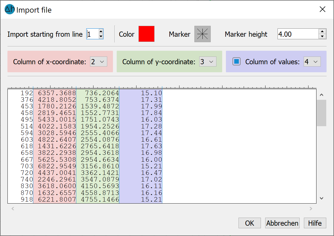
The measured values and the location of the measuring points can be displayed at any time via File Import Overlay file *.txt. The data is selected via the following input window.

Firstly, click on the "Preview" button. The columns are then selected in the lower area of the dialogue. A marker (type, height and colour) can also be selected).

Import text file

After successful interpolation, the calibration potential heads can be displayed via the View Show Attributes Attributes… or by clicking the Isolines/area plots/values... toolbar button. Display the EICH values using isolines with the interval 12.50 to 20.0 and the distance set to 0.5 m):

 

Interpolated calibration potential heads, isolines at a distance of 0.5 m

 

In the upper reaches of the stream, the previously described but not actually existing groundwater infiltration of the stream can be recognised, which is made visible by "groundwater mounding". The data is processed as follows for the calibration:

First, the VORF attribute is copied to an auxiliary data type (e.g. KKKK, if already assigned, then delete beforehand!). The VORF watercourse water level (stage) elevations are deleted at 17 nodes of the upper course of the stream (Attributes Delete... and then selecting VORF and Polygon).

Then the current EICH potential heads must be completely deleted. After the deletion of EICH, the modified VORF watercourse stage elevations and the POTE potential heads are then copied to the EICH attribute again. The interpolation of the calibration potential heads described above must now be repeated.

 

Interpolated calibration potential heads taking into account the receiving water conditions

 

The complete VORF watercourse water level (stage) elevations stored on the auxiliary attribute (e.g. KKKK) can now be reassigned to VORF (Attributes Copy Attribute method...).

 

Due to the low data density in the area of the abstraction wells, their lowering of the groundwater table is not reflected in the course of the isolines.

The terrain elevation must also be assigned via interpolation. Terrain elevation are often available as ASCII data records, which must first be read into the structure data file.

The file "s3_gela.zip" is included along with the files provided for this tutorial (relative directory: .../Tutorial_bsp_files/Tutorial_2D_bsp_files/s3_gela.zip). This zip file contains the file gela.txt. As this file is not in the structure data format (p. 35), this data must first be imported as a structure (Structure Import…). The data can then also be assigned via Attributes Assign By interpolation..., Input: Structures Add.

 

 

The next step is a Manual attribute assignment