The attribute menu is only available in the model mode. The following menu items are available:
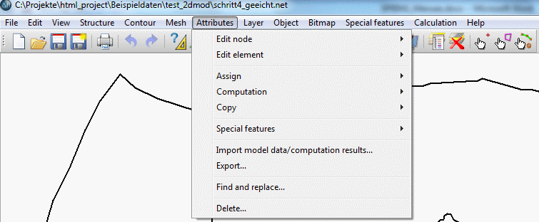
Edit node
The node to be edited can be selected either by its number or by capturing it or by using the button  of the toolbar. The selected node is then marked and the input window where the attributes of the node can be edited appears on the screen:
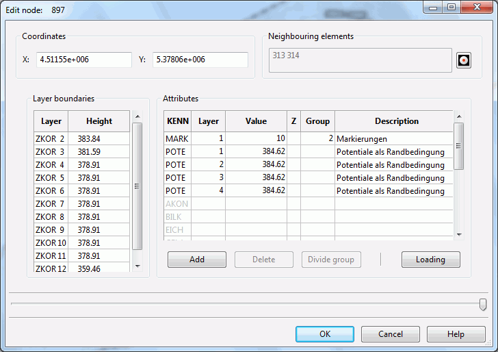

Coordinates:
The text boxes containing the x- and y-coordinates of the present node make it possible to edit the coordinates directly. But be careful, and do not move the node too far from its original position. Otherwise, the elements to which the node belongs to could be distorted. The attributes assigned to the node will stay the same regardless of whether the coordinates are changed.

Neighbouring elements:
The box Neighbouring elements contains the numbers of the contiguous elements of the node. By activating the button  zooms the representation to the selected node.

Layer boundaries:
Here, the geometric data are displayed, e.g. the ground level as the upper layer boundary or in a 3D model, the heights of the Z-coordinates.

Attributes:
The attributes of the node can be added (left button), deleted (right button) or changed by manually editing the cells of the table (value, group or attribute sign (Z)). After opening the model, the node attributes are not loaded yet. At first, the attribute to be edited has to be marked. Then the button "Loading" is activated. After pressing the button the corresponding node values are read in from the model file and can be edited.
First, all in the model file existing node attributes are shown. Is a selected attribute at that node non-existent, the entry disappears after clicking the button "Loading".

Divide group:
If the node has got a group attribute like LERA or MARK and the attribute is selected in the dialog the button "Divide group" is activated. After pressing the button the attribute group is split at the subsequent node. The following node is derived from the original allocation direction. A new group is then created automatically for the following nodes.
If the window is closed with OK, all modifications of the node data are stored. The modifications can be undone with Undo  .
.
If the window is closed with Cancel, all modifications are ineffective: the node data remain as they were before opening the input window.
Edit element
The element to be edited can be selected either by its number or by capturing it or by using the button  of the toolbar. The selected element is then marked and the input window where the attributes of the element can be edited appears on the screen:
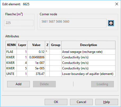

Corner nodes:
The box Corner nodes contains buttons for the nodes associated with the element. By activating the button  zooms the representation to the selected element.

Attributes:
The attributes of the element can be added (left button), deleted (right button) or changed by manually editing the cells of the table (value, group or attribute sign (Z)). After opening the model, the element attributes are not loaded yet. At first, the attribute to be edited has to be marked. Then the button "Loading" is activated. After pressing the button the corresponding element values are read in from the model file and can be edited.
First, all in the model file existing element attributes are shown. Is a selected attribute at that element non-existent, the entry disappears after clicking the button "Loading".
If the window is closed with OK, all modifications of the element data are stored. The modifications can be undone with Undo  .
.
If the window is closed with Cancel, all modifications are ineffective: the element data remain as they were before opening the input window.
Assign
Since this menu item is very complex, it is treated in a separate chapter.
Computation
Since this menu item is very complex, it is treated in a separate chapter.
Copy
Since this menu item is very complex, it is treated in a separate chapter.
Special features
The following submenu appears:
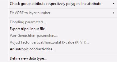

Check group attribute respectively polygon line attribute
By using this menu item can be checked if existing attributes (single or all) with group or polygon data overlap with similar attributes.
Input window Single attribute:
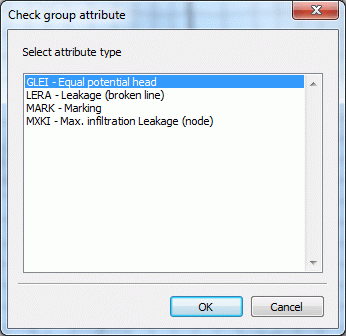
As a result, the overlapping group or polygon data are shown as green lines. The nodes on which attributes are defined twice, are marked by a green circle.
Via the menu item Attributes  Edit node
  Capture these nodes are selected and in the appearing input window the corresponding groups are deletd.

Fit VORF to layer number
This menu item is only available in a 3D model in which the attribute VORF is assigned. You can choose between two possibilities: by equal potentials or by moving.
By equal potentials:
This procedure is perfect for discharge system data sets which describe a discharge system near the surface. The following query appears:
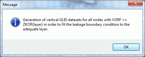
If a 3D-modell is discretized relative fine in vertical direction the discretization is not sufficient in most cases for a discretization of the correct terrain decrease at a discharge system. Here the mesh nodes on the discharge system in the top layer normally hang in the air that is above the water level (see the lower figure). In this case it makes sense that nodes beyond the level are set equal so that the leakage boundary conditions reach at the correct position.
For this it is simplest to assign the attribute VORF and the corresponded leakage coefficients (LERA or LEKN) on the first layer. By activating the function Fit VORF to layer number  by equal potentials a vertical GLEI-data set will be generated from the among each other laying nodes where the input for the discharge system potential (VORF) is greater than or equal to the Z-coordinate of the node.
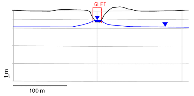
GLEI-nodes at a discharge system (vertical section)
By Moving:
This procedure is perfect for discharge system data sets which describe a leakage boundary condition "inside" (e.g. ducts):
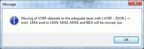
With this procedure the Z-coordinate is determined where the distance to the VORF value is at minimum. By activating this function all data types of a VORF-node which correlate with the discharge system node boundary condition (VORF, LERA, LEKN, MXKI, MXKE and BILK) are removed to the corresponding adequate layer!

Flooding parameters…
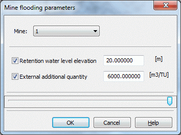
If the attribute GRUB (balance nodes for mine flooding) is assigned, the water level and the additional amount of water for the individual mines are defined in the following input window. A detailed description can be found in the "How To – Simulation of flooding processes“.

Van-Genuchten-parameters…
If the attribute USAT is assigned in the model file, the parameters of the individual saturation regions are defined using this menu item:
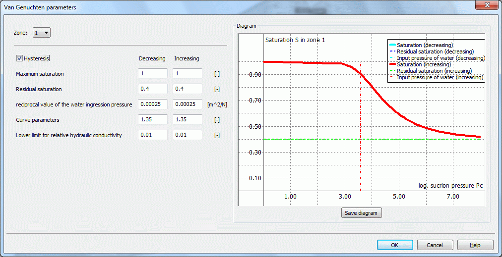
This menu item and the corresponding input window are described in chapter: „Data structure of the groundwater model – Saturation parameters, Hysteresis“ in detail.

Adjust factor vertical/horizontal K-value …
The following input window appears:
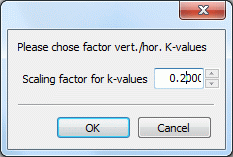
By using this function you can change the ratio between the horizontal and the vertical permeability used in 3D models. The default value is 0.1.

Anisotropic conductivities …
Since this menu item is very complex, it is treated in a separate chapter.

Define new data type
The following input window appears:
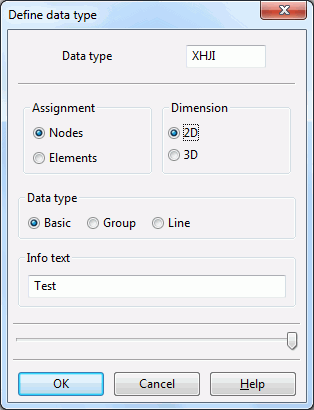
Here new data types can be defined, which are not registered in the file xsusi.kenn. Details can be found in the notes in the chapter "Information of the file xsusi.kenn".
Import data/computation results…
By using this function you can import model data from other directories or calculation results from the different SPRING modules. First, a file selection box appears:
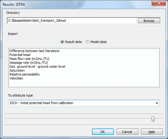
You must specify the directory where the calculation was carried out or in which the model data is found. (SPRING does not check whether the data existing in the binary files fit to the current project.)
The box Import contains a list of result data types where you can select one. The box To attribute type defines the identifier where the imported data in the current model are assigned to. For all data types except the velocities, you can define any ID-code, even identifiers unknown to SPRING. An acceptable ID is a combination of 4 letters or numbers (underscore is also allowed).
Depending on the selected result data type, SPRING automatically knows whether to save the data as nodal or elemental data. For the case of velocities, it is not possible to define an individual identifier, because the values are automatically assigned to the elemental data VV_X, VV_Y and eventually VV_Z.
By confirming the menu with OK, the selected results are imported and assigned to the corresponding nodes/elements in the appropriate layer of the current project.
Export…
By using this function, you can create an ASCII file containing formatted data directly in SPRING. The available format is the STR-format (I6, F10, F10, F10).
The following window appears:
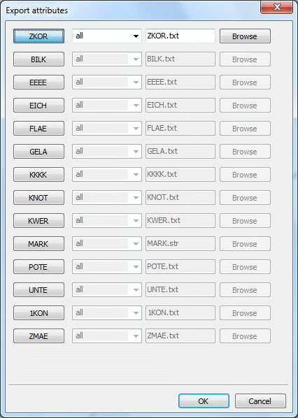
By clicking on one or more buttons the attributes to be exported are selected. Subsequently, the desired layers in a 3D model and the name of the output file are specified. With the button Browse a different directory in which the data should be stored can be selected. By clicking on the OK button the export starts.
Find and replace...
Using this menu item, attribute values or attribute characters in one or all layers (3D model) are automatically replaced in the model file. A possibly existing attribute character will not be automatically replaced with, but must be specified explicitly.
The following input window appears:
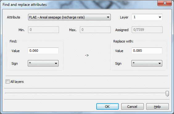
For orientation, the minimum, maximum and the number of assigned values are given. With the checkbox "All layers" values can be simultaneously found and replaced in all layers.
Delete…
By using this function existing attributes can be deleted. It is possible to delete either a single attribute or several attributes simultaneously:
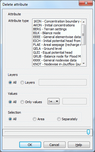
In case of a 3D model you can delete the data either in all layers or only in one single layer.
You can decide whether all values or only a certain value, in the whole model (all) or only in a certain area defined by a polygon or separately should be deleted. The different options can be combined any way you want (e.g. "only POTE in layer 3 in a certain region" or "only LERA in a certain region with the value 200.0" ...).
Only the values of nodes or elements are deleted that are entirely within the selected polygon.
