This menu item contains all display options that are possible for attributes. If a sub-item listed in this menu is not included in the model, then the sub-item is deactivated in the menu, i.e. it appears grey.
Attributes… 
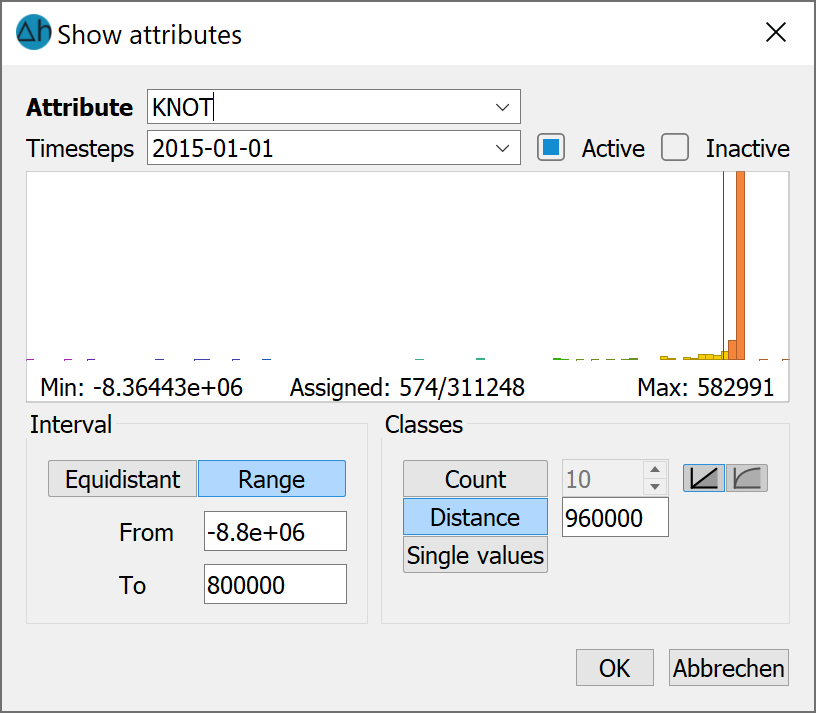
This menu item can be used to create isoline, coloured area, circle or line displays of node and element attribute data. A list of all assigned node and element attributes is provided and the type of display can be defined. After clicking on the menu item, the following input window appears:
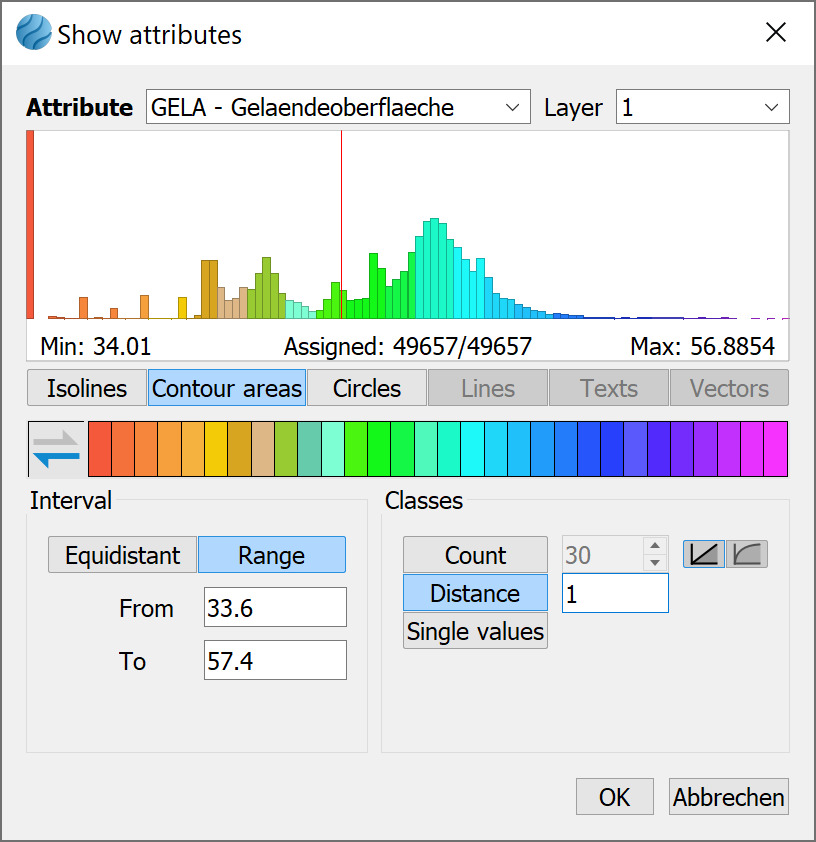
The colours of the distribution curve in the preview window interactively show the colour distribution of the selected interval range. The arrows next to the color scale can reverse the palette.
Attribute (identifier, information)
The attribute to be displayed is selected here based on its identifier. For a 3D model, it is also necessary to select the layer number. If a 2D data identifier (e.g. terrain height) is selected for display, the layer number is automatically set to 1 and cannot be changed.
The min/max range beneath the histogram plot indicates the minimum and maximum value of the selected attribute. The “Assigned” value indicates how many of the nodes or elements are assigned the selected attribute in relation to the total number of nodes or elements.
Type of presentation
You can choose between:
Isolines plot with determination of the colour
Contour areas plot (for node data these are coloured areas between isolines, for element data this is a colouring of the element with a colour dependent on the element value).
Circles plot in which a coloured circle marker with a radius depending on the value is displayed in each element or at each node. The circles have a minimum radius of 6.0 (pixels). The height of the circle for the largest value found can be set in the max. radius field. If all circles are to be the same size, a radius of 6.0 must be selected as the max. radius.
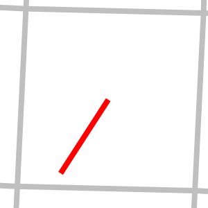
Lines plot, recommended for attributes that are primarily assigned along a line (e.g. polygonal leakage values or equal potential heads along a lake edge)
There is a special feature for the "Velocity vectors" data type [m/TU]. These are only displayed once they have been imported via the Attributes → Import model data/result data… menu item. In addition to the individual direction components (VV_X, VV_Y, VV_Z), a resulting velocity vector VVEC can be displayed. The associated values correspond to the imported result attribute VMAG.
The following options are available:
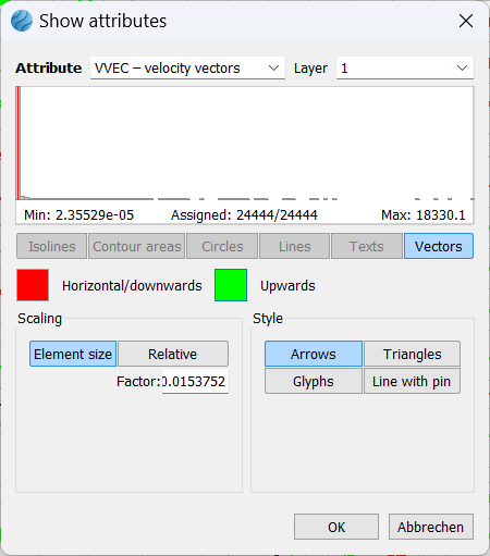
Firstly, the vectors can be scaled:
The flow arrows can be scaled according to the size of the velocities. This form of representation is similar to the representation of velocities in the plot generation. The greater the velocity, the longer the vector, which is displayed with the arrowhead at the element centre point. If the velocities are too small, the vector is displayed with a minimum length.
Alternatively, it is possible to automatically scale the velocity vectors so that they fit into the associated element as far as possible. In this form of display, the arrow shown only represents the direction of the velocity, not its size. The vectors shown are displayed with a length of 80% of the average element edge length and are plotted with their centre point in the centre of the element
There are four different display styles:
Triangles
Arrows

Glyphs
Line with pin
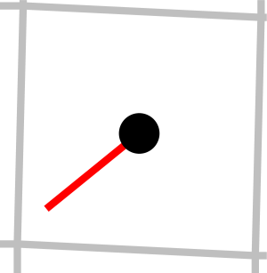
The display styles as glyphs or lines with a pin are similar to a wind vane: The starting point is in the centre of the element, the line is then aligned by the flow.
Value interval and classes
Various display options are available for the value range of the selected attribute:
If Equidistant is selected as the interval, the values are obtained from an even division of the range of values found (minimum to maximum). The Count (number) of subranges is entered in the text field under Classes.
With the Range division type, the interval defined by means of the From and To text fields under the Range option is divided evenly when using the Count classes option. The number of divisions is entered in the Count text field. It is possible to make a logarithmic subdivision by activating the Logarithmic graph icon to the right of the Count classes option (recommended for K-value intervals, for example).
With the Range division type, the interval can also be subdivided by a fixed number by mean of the Distance classes option. This option divides the intervals by means of a fixed number between each interval.
If Single values are to be entered, an input field appears for the desired number of intervals and a table in which the interval limits can be defined individually. A colour can also be selected for each interval.
If the display attributes are selected, the selected data is stored in a special layer. This layer is listed in the project manager and can be shown or hidden there. In addition, the legend of the layer can be shown by activating the corresponding checkbox.
Attribute token…
This menu item can be used to display the nodes or elements that have been assigned an attribute token (character in the 15th/16th column of the model file) (e.g. all receiving water nodes that have been assigned a fixed value by means of the character F). The following dialogue window appears:
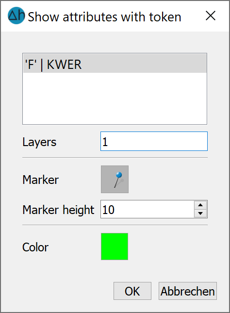
All attributes that are assigned a token character are listed. A layer selection is possible for 3D models. The type of marker, its height and colour must also be specified.
Transient… ![]()
Please note that transient data can only be displayed after it has been imported via the Extras  Transient Import input file… menu item.
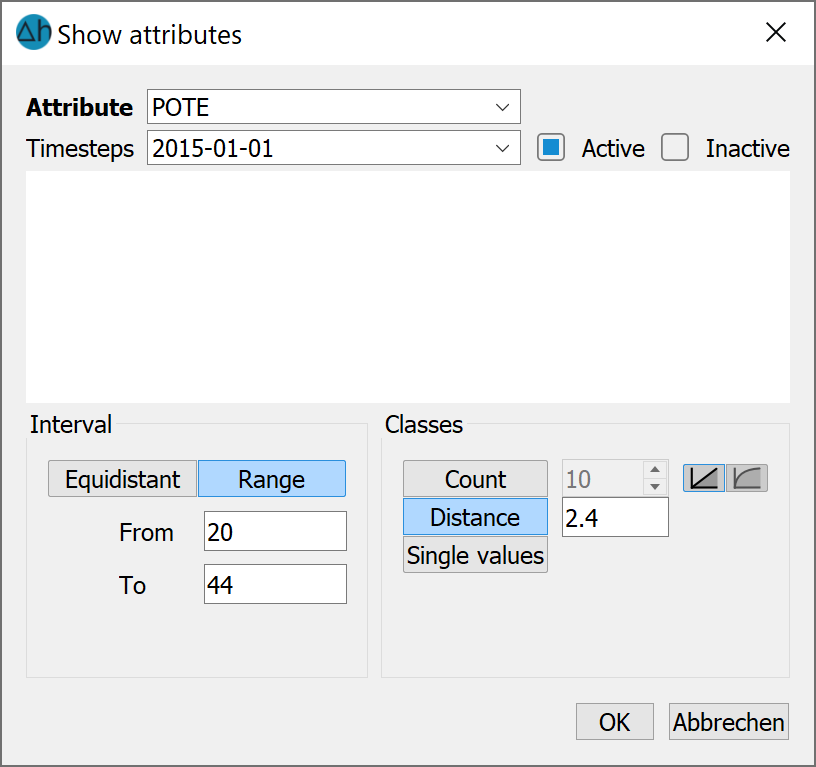
After selecting the View → Show attributes… → Transient… menu item, the following input window appears:
In the Attribute drop-down box, the transient attributes from the transient input file are displayed. Depending on the selected attribute and the time step, the existing minimum and maximum values and the number of occupied nodes or elements are displayed. The desired layer can be selected for a 3D model.
By selecting the active/inactive checkboxes, you can differentiate between the nodes/elements that are active or inactive for the selected properties. Active means, e.g. for the identifier POTE, the potential head at this node is kept at the specified value for this time step. A node is inactive if it is labelled with a minus in the transient input file. For the previous example, the potential head boundary condition is then switched off at that particular node for the specified time step.
The nodes or elements that are assigned with the selected transient attribute and time step are displayed (circular plot) when the dialogue is closed with OK.
Hydrograph 
Once a transient input file has been imported via Extras Transient Import input file…, the data can be displayed as a hydrograph by selecting the View Show attributes… Hydrograph… menu item and selecting a node or element with the corresponding attribute. The hydrograph then appears for the selected object:
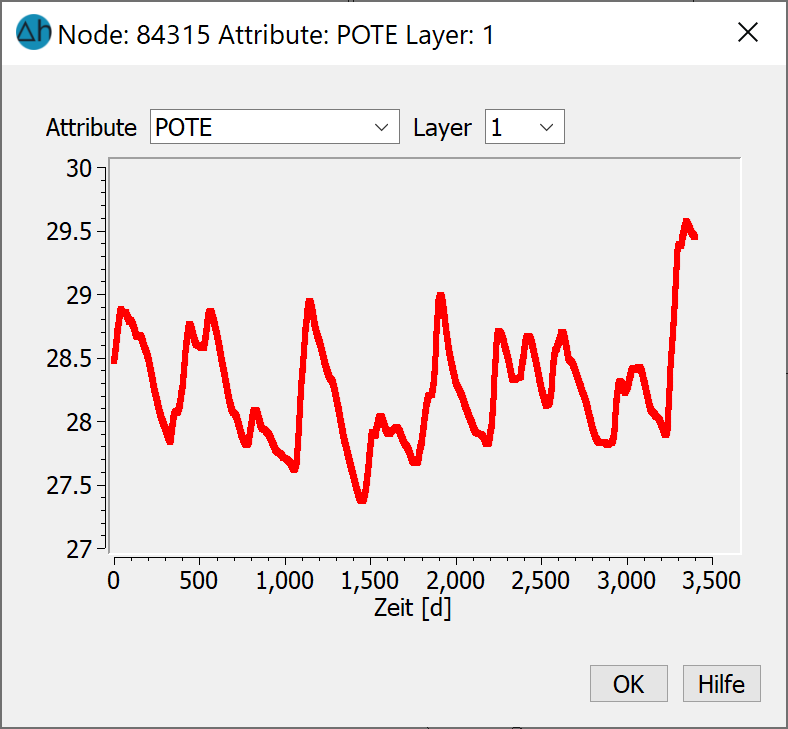
If different transient data are available or transient data are defined in several layers, these can also be selected
Node texts/element texts
By selecting this menu item, the node or element texts specified in the mesh and/or 3d file are displayed. Alternatively, node or element texts can be displayed via the Attributes… () menu item and selecting the data type KTXT or ETXT. When using the Attributes… menu item, the appearance of the text can be modified.
Stand: 06.03.2026 | 