Call up via selection in the menu from File  Create plot Top view/map presentation...
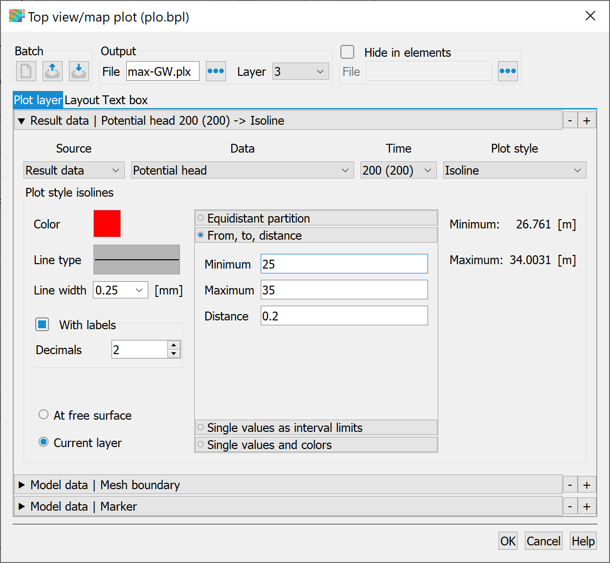
After selecting this menu item, the following input window appears:
The buttons at the top of the input window allow you to reset the input parameters ( ), open an existing batch file (
 ) or save the current batch file under a different name (
 ).
).
Output
(batch command DATE)
The name of the output file is defined at this point. The name of an existing *.plx file can be loaded via the file selection window.
For a 3D model, you can select the layer for which a top view is to be created (horizontal section).
Hide in elements
For some models, it may be useful not to display the results (e.g. velocity arrows or isolines of the potential heads) in certain model areas, e.g. because the GWL is unsaturated or does not exist as a conductor in the selected layer of a 3D model. The area to be hidden is defined in a separate ASCII file (Hide) by specifying the corresponding element numbers. The format of this file corresponds to the "Input format of the mesh file" (16x, 9 (I6, A1), A1) starting from the first line without any data identifier or comment line, whereby the data value is arbitrary or can be missing.
If the Hide in elements checkbox is activated, the file name of the hide file must be specified or can be selected using the Open file button
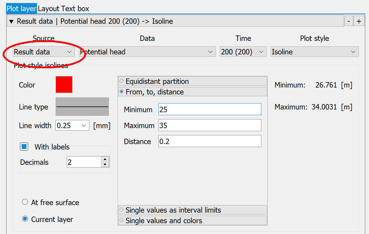
Source, data, time, plot style
The individual layers of the subsequent plot are selected and compiled in this area of the input window.
The order in which the layers are selected is not relevant. Before the plot file (*.plx) is created, the layers are sorted so that background representations (raster, polygons, continuous results data like potential heads) are placed behind point or linear representations. The active layer is indicated by the arrow pointing downwards.
Using the buttons to the side of the display type

it is possible to add further layers (+ button) or remove a layer from the list (- button). Th - button removes the active data record from the list.
The selection field in the Source column offers the following options:
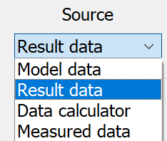
Depending on the selection in this field, there are further input options for the other columns (data, time and plot style).
Source: model and result data
When selecting model or result data in the selection field of the source, the data types saved in the background files are provided in the selection field in the Data column. The data types for the model data result from the attributes available in the model file, and for the result data from the previously performed calculation. After a steady state flow calculation, for example, this result data is available:
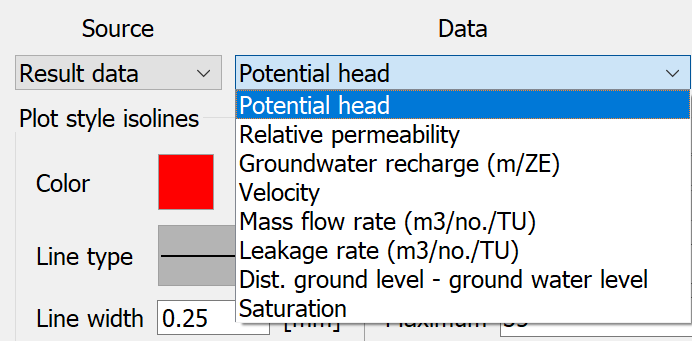
With a transient calculation, the timestep to be displayed can also be defined.
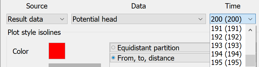
The selection of the data type results in corresponding or different display options. The following display types are available for area-wide defined element data.
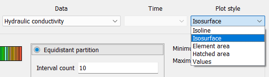
The hatched area display type is only possible for element data.
The following display types are available for node data, which is often defined in a comprehensive manner:
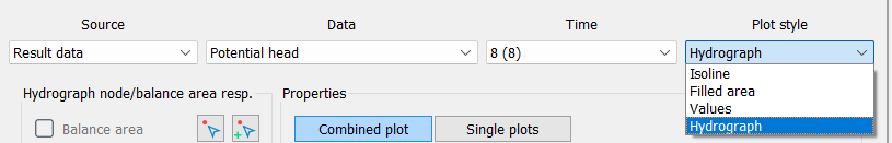
The hydrograph display type is only possible after a transient calculation.
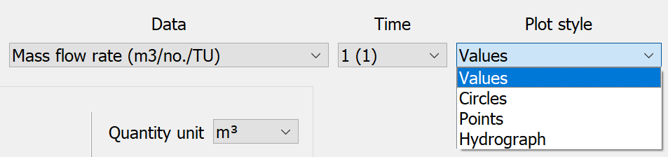
The following visualisations are offered for point data such as sources/sinks or fixed potential heads:
For special data such as element/node numbers, mesh, mesh edge or markings, only the line display type is offered, which can be modified as required in the Line plot input block.
Source: Data calculator
Here it is possible to combine data from the same or different calculation runs or from other layers in 3D models and then display them (batch command RECH).
In addition to the Plot Style input block, the Data sets input block is also visible:
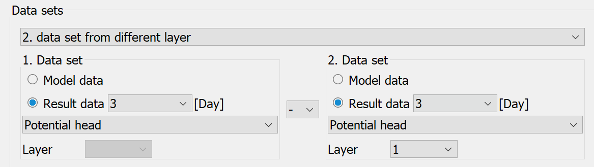
Firstly, the model/results data basis on which the data is to be calculated must be specified. The following options are available:
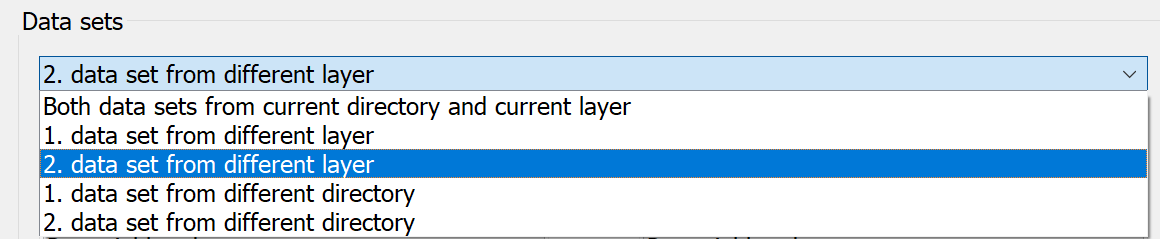
Both data sets can be from the current directory, i.e. from the same calculation run, and (in the case of a 3D model) from the current layer.
Both data sets can be from the current directory, i.e. from the same calculation run, but one of the two data sets can be from a different layer (in the case of a 3D model).
Both data sets can be from the current layer (in the case of a 3D model), but one of the two data sets can be from a different directory, i.e. from a different calculation run.
If a data record from another directory is to be used, the path relative to the current directory to this directory must be entered in the text field (alternatively, the directory can also be selected using a file selection window).
If a data set from another layer (3D model) is to be used, the layer number must be entered in the corresponding text field.
If Data calculator is selected, the Data and Time selection fields cannot be edited. These two necessary pieces of information are defined in the Data sets input block for both data types.
The 1st data set is defined in the left-hand section of the above input screen and the 2nd data set for calculation is defined in the right-hand section. After selecting whether model data, result data or, if applicable, result data over time (transient calculation) should be used, the actual data types must be selected. In the case of a 3D model, all data always refers to the layer number specified in the Output input block, unless data from another layer is being calculated!
If you select to perform a calculation using two data records, they can be linked with the four basic arithmetic operations addition (+), subtraction (-), multiplication (*) or division (/).
Possible display types are: Isoline, Filled area or Values:
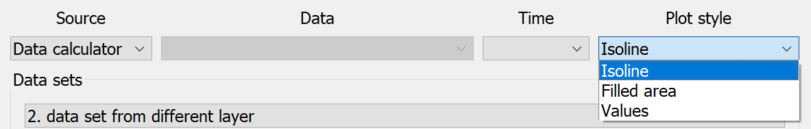
The display parameters are defined in the Plot style input block.
Source: measured data
If measurement data is to be displayed, the Measured data parameters input block appears. If Measured data is selected, the Data, Time and Plot style selection fields cannot be edited.
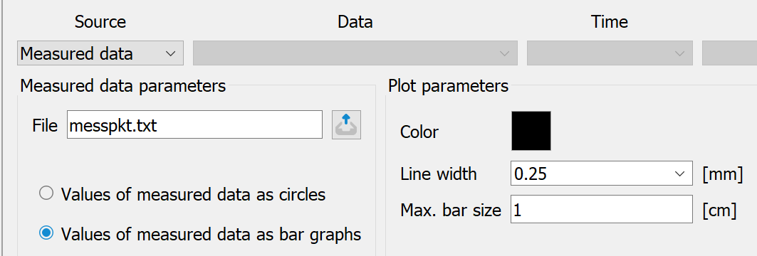
The measured data input block has the following input options (batch command EICH):
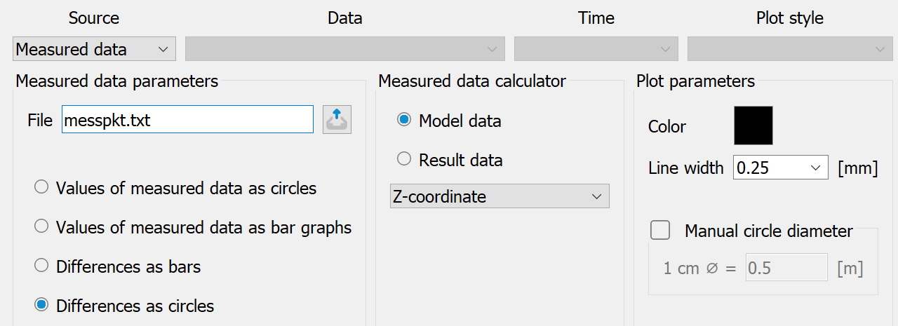
Firstly, the name of the measurement data file is entered or selected in a file selection window. The measurement data file can only be analysed if it is available in structure data format.
The following options are available for displaying the measurement data:
Display the values of the measured data as circles:
The measurement points are marked with a + marker and the values are plotted at the points (see plogeo.ini commands EHGT and ETYP ). The marker type is defined in the plot options. A colour and line width can also be selected.
Display the values of the measured data as bar graphs:
Bar graphs are plotted at the measuring points. The bar height indicates the value of the measuring point. A colour, a line width and a maximum bar size can be selected as further inputs. The specification of a maximum bar size is a type of scaling for the measured values:
Difference between the measured data as bar graphs or circles and any model data or result data type:
If these options are selected, the measurement data is compared with an existing data type (model or result data). A difference is formed and plotted as a bar or circle. In addition to entering a colour, a line width and a maximum bar size (see above) or a circle diameter, a data type must be selected (possibly also a time step) with which the measurement data is to be offset (plogeo.ini command RADI ).
For a 3D model, the difference is made for the layer specified under Output. Plot parameters for their circular representation:
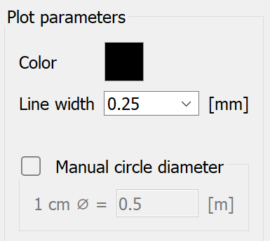
If manual input is not activated, the maximum circle size is defined via the options in the plogeo.ini file (Edit Preferences…). The batch file for plotting then contains the following for EICH, for example:
EICH ## Measured data differences as circles
201 0 0 0 1 0.5 # Potentials
1 0.25 0 0 # Colour, line width, circle plot
gwmesspkte.txt # file with measured data (structure file format)
The digits of the values at the measuring points are converted into polylines. The height of the digits is 0.18 cm by default and can be changed in the Edit menu Preferences Plogeo Size (plogeo.ini command HWER ).
If the corresponding checkbox is activated in the plot options, an ASCII file DiffEich.txt is created when the measurement data is offset against other data, in which the x and y coordinates, the difference, the measured value and the calculated value are saved in the format (6X, F10.2, F10.2, F10.3, F10.3, F10.3). This file can be used to create a scatter plot (measured/calculated values as an x/y diagram), e.g. with Excel.
The details of the representation of areas, hatching, isoline etc. are described in the chapter "Presentation types".
The settings for the layout and text field are described in detail in chapter "Advanced settings".
Stand: 02.06.2025 | 