After navigating to Calculation Inverse calibration and selecting the calculation type from the following menu:

 

 

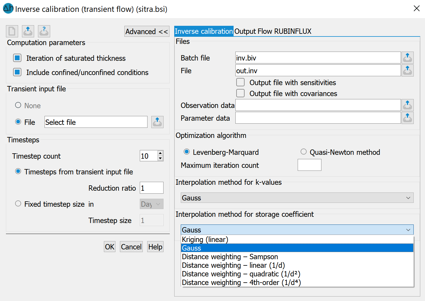
The respective input windows of the selected calculation module and the tab pages with the extended settings for inverse modelling appear. The required entries for inverse calibration are independent of the selected calculation type. The following illustration shows the tab pages for inverse calibration.

When the input screen is called up, the programme reads in the batch file with the preset names sitra.bsi and inv.biv (if they exist). The default settings in the mask are changed accordingly.

 

Files

An inverse modelling run requires two batch files: The "normal" batch file with the control parameters for the direct problem (default: sitra.bsi) and a batch file with the control parameters for the inverse problem (default: inv.biv). The latter is defined here.

An inverse modelling run generates two output files: The first output file contains the results of the last calculation run of the direct problem (out.s). The second output file is defined in this dialogue (default: out.inv) and contains the log of the inverse calculation run with error tables for each iteration step and an output of the optimised parameters. If the "Output file with ..." checkboxes are activated, the sensitivities (files param_name.sns, out.inv_tab.csv and out.inv.sens) and the covariances (file covariance.csv) are written to additional output files.

The sensitivities provide a statement about how a change in the i-th parameter pi in the current parameter set p affects the calculation result in the j-th observation date bj.

Covariance is a measure of the (linear) correlation between two random variables with a joint distribution. The covariance is positive if a and b tend to have a linear relationship in the same direction, i.e. high values of a are associated with high values of b and low values with low values. In contrast, the covariance is negative if a and b have an opposite linear relationship, i.e. high values of one random variable are associated with low values of the other random variable. If the result is 0, there is no linear relationship between the two variables a and b (non-linear relationships are possible) (from Wikipedia).

In inverse modelling, the covariances of the parameter values are calculated and compiled in tabular form in the covariance.csv file.

The files with the observation and parameter data must also be specified.

 

Optimization algorithm

The Gauss-Newton method according to Levenberg-Marquard and a quasi-Newton method are available as optimisation algorithms.

The maximum number of iterations can be specified in the text field, at this maximum value the optimisation algorithm will be terminated regardless of the state of convergence.

 

 

Interpolation algorithm

The parameters for any necessary interpolation of K-value parameters or storage parameters within the respect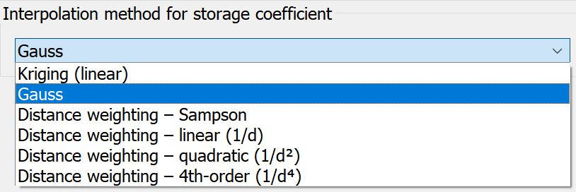ive zones (Z-KW or Z-SP) are defined here. The following interpolation algorithms are available:

 

In contrast to the Interpolation calculation module, a maximum search radius for the interpolation points is not required for distance weighting. The maximum number of points with the smallest distance specified in the text field is always used for the interpolation.

 

Results