It is recommended that you first carry out a run with 0 iterations. This allows the target function to be checked without much effort or time. The results are written to the output file (here: out.inv), whereby the proportions are listed individually for each parameter/measured value group.

It is important to balance the proportions of the target function. After the first inverse calculation run (0 iterations), the proportions of the target function can be compared with each other. The best known variables (usually potential heads) should have the largest share of the objective function (ZF).

 

Possible sources of errors:

• K values are too heavily weighted. This means that the algorithm is not permitted to calculate the K value far from the estimated value, and there are almost no changes in the distribution of the hydraulic conductivity.

Remedy: Increase standard deviations

• Rates are weighted too heavily. As a result, the measurements of the potential heads lose weight and the algorithm tries (in vain!) to bring the rates into agreement. In most cases, the following rule applies: If the potential heads and the K values are correct, the rates should also match.

Remedy: Balance the weighting proportions of the target function (by means of well chosen standard deviations)

• Transient measurement series: Piezometer x is measured every day for a year, whereas piezometer y is only measured once a month. If all individual measurements have the same σ (i.e. are weighted equally), the groundwater measuring point x will be a total of around 30 times more heavily weighted than the groundwater measuring point y (365 measurements compared to 12 measurements)).

Remedy: Select smaller σ for piezometer y

 

If the proportions of the target function are balanced, the number of iterations is set to 10 and inverse modelling is restarted.

 

Output files

• out.inv

File with calibration history (measured/calculated values/target function) as well as the K values and leakage factors in the format of the model file. The iterated K values can be stored directly on the KWER attribute via Attributes Import model data/result data....

• Invpar.csv:

File in the format of the parameter file (note: semicolon as column separator, point as decimal separator). The calculated K values are listed in column D. This file can be renamed and then used as an input file for a next run (e.g. with partially recorded values).

• Invpar_xy.csv:

Analogous to invpar.csv, however coordinates are included (not for LERA!). The file can be overlaid, for example, to visualise the results.

• resan_pote.csv, resan_lkno.csv, resan_knot.csv (steady state only):

Contains all data on the measured values. Replace “name” with the attribute identifier, for example: resan_pote.csv, resan_lkno.csv, and resan_knot.csv

 

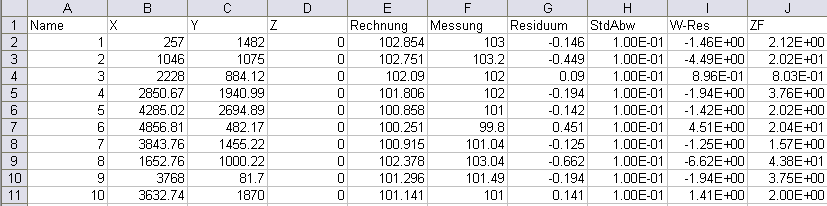
Example of the resan_pote.csv file

 

 

• name.csv (transient only):

For each measuring point (POTE, LKNO, KNOT) a *.csv file with the time varying data is written out. As no distinction is made here between data types, it is important to clearly define the names in the observation file (*.obs). For example, do not designate a potential head as X1 and a rate measurement also as X1. It is better to clearly distinguish between the different attributes by, for example, designating the variables as h_X1 and q_X1.).

 

Example of a transient output file name.csv

 

Batch files