Preparation in the model file

The parameters to be calibrated must first be defined in the model file. For example, stream sections are summarised, or the hydraulic conductivities are divided into zones.

Within a zone, either a single K value or storage coefficient (number of parameter values within the zone = 1) or an array of K values or storage coefficients (number of parameter values within the zone > 1) can be calibrated.

For the calibration of leakage coefficients, the surface waters must be available as LERA. A river or stream can be divided into several sections; these sections must be the same for LERA and Z-LR. Only one value can be specified and optimised within a section.

 

Structure of the parameter file

The parameter file must be in *.csv format. The columns are separated by a semicolon (semicolon) and the point is used as the decimal separator. The structure of the file is as follows:

 

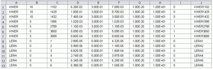
Example of a parameter file

 

• The type of parameter is defined in column A. The following types of parameters are currently implemented in inverse modelling: KWER, KSPE, LERA, FLAE.

Zones can be defined in the model file (Z-KW, Z-SP) for the calibration of KWER and KSPE by area. Ideally, these should correspond to the geological formations within which uniform parameters are to be expected. If only one formation is present, a single zone is defined.

• The zones of the Z-KW and Z-SP are entered in column B. Column B always contains 0 for the LERA parameter. The assignment with Z-LR is made in column C.

• The element number of the interpolation point is defined in column C.

• Column D is the start value for the respective parameter. This value is read in during the first inverse calculation run.

• Column E contains the standard deviation. This corresponds approximately to the expected error of the size. For potential head measurements this can be 5-10 cm, for rates 10% is a good value. For logarithmic rates such as KWER, the standard deviation is given in orders of magnitude (for example: K value = 1e-03 +/- 0.5 orders of magnitude).

• Column F contains the estimated value of the parameter for the generation of the residual.

• Column G/H contains the lower and upper limits of the estimated value from column F.

• Column I contains a 0 for variable values or a 1 for fixed values (make sure that the desired value is defined in column D!) → The effect thereof is shown in the following illustration.

• Column J contains the name of the parameter that appears in the output file.

 

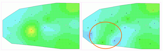
Support points and initial K values. Right: The area of the variable K values is circled (column I=0). The K values at the other sampling points are retained (column I=1), but must still remain in the parameter file so that the interpolation can be carried out

 

 

Structure of the observation file

The existing measured values are saved in a file without a special format (e.g. text file). The structure of the file for steady state and transient measured values is as follows:

 

Line 1-3 comments

Line 4 empty

Line 5 ZEITEINHEIT MENG SEKUNDE (MINU STUN TAG_ JAHR)

Line 6 ZEITEINHEIT ZEIT SEKUNDE (MINU STUN TAG_ JAHR) OR

Line 6 BEZUGSDATUM XX.YY.ZZZZ

Line 7 empty

Line 8-x measured values:

 

POTE Name_1 // comment (Attention: no space in the name!)

x-coordinate y-coordinate [z-coordinate in 3D]

Zeitpunkt Measurement Standard deviation OR

DATUM Measurement Standard deviation

 

KNOT Name_2

Number of nodes n

n node numbers (10 per line)

Zeitpunkt Measurement (Sum over all n nodes) St.dev. OR

DATUM Measurement (sum over all n nodes) St.dev

 

LKNO Name_3

Number of nodes n

n node numbers (10 per line)

Zeitpunkt Measurement (Sum over all n nodes) -St.dev. OR

DATUM Measurement (Sum over all n nodes) -St.dev.

 

The time units for the rates and the time unit for the time scale are defined in lines 5 and 6. For steady state measured values, the time unit is specified as TIME with the time 0.0 in the file. For transient measured values, you can select whether to work with an absolute time scale in a time unit (example hour: 0.0, 1.0, 1.5, 2., 20.) or with a reference date and thus with a date time scale.

The measured values follow from line 8. There are 3 possible categories: POTE for potential head measurements, KNOT for point withdrawal/injection rates and LEKN for measured infiltration/exfiltration rates over a section of a stream. The control word for the category is followed by the name of the measuring point. Care must be taken to ensure that there are no spaces in the name. No tab should be used between the x and y coordinates.

The time is followed by the measured value of the variable and the standard deviation of this measured value. The standard deviation is required for weighting the measured value. This variable and its function are discussed in more detail in the chapter "Minimisation of the target function".

To illustrate this, examples of a steady state and transient observation file is provided below:

 

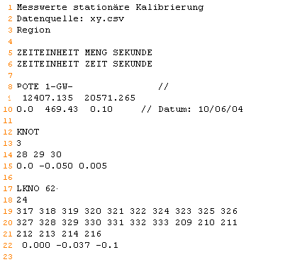
Observation data for the steady state calibration

 

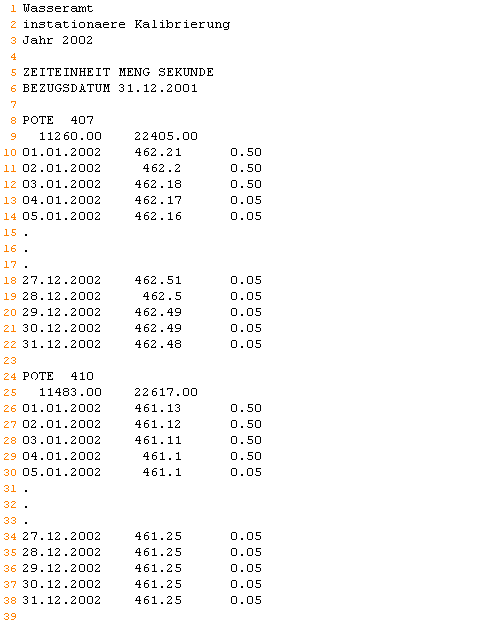
Observation data for the transient calibration

 

Input parameters