Minimization of the target function

The aim of inverse modelling is to minimise the target function. The target function is made up of two main components:

ZF = ZF_obs+ ZF_par

Both the measured values (ZFobs, e.g. potential heads, rates) and the estimated values of the parameters (ZFpar, e.g. K values, leakage coefficients, storage coefficients) are included in the target function. The proportions are further divided:

ZF_obs = ZF_POTE + ZF_LEAK + ZF_KNOT

ZF_par = ZF_KWER+ZF_LERA + ZF_KSPE

To determine the target function, each parameter and measured value is assigned a standard deviation σ. This corresponds approximately to the expected error of the variable.

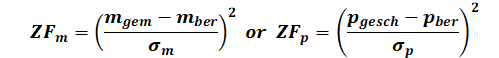
Each measured value m and each parameter value p is analysed after each step of the inverse calibration as follows (least squares method):

For the numerical solution of this non-linear minimisation problem, two different mathematical algorithms are offered for inverse modelling in SPRING:

a Gauss-Newton-method according to Levenberg-Marquard and

a gradient method according to the Quasi-Newton-method

The target function components of each measured value and each parameter are totalled. If a small standard deviation σ is selected, this results in a large proportion of the target function and therefore a high weighting. A large standard deviation σ results in a small proportion of the target function and therefore a small weighting.

The following table shows the influence of the weighting.

The two potential heads H1 and H2 are listed first. The residual is the same for both measuring points, but there is a hundred times greater proportion of the target function for H2, as this value is weighted more heavily with 10 cm standard deviation than H1 with 1 m standard deviation.

Another effect can be illustrated with the rates Q1 and Q2. Depending on the unit in which the calculation or evaluation is carried out, a different weighting results for the same standard deviation).

Therefore, standard deviations in the range of 10-25% of the measurements (depending on accuracy) should always be selected for rates. Q1* and Q2* have a standard deviation of 10% - the proportions of the target function are of the same order of magnitude.

A parameter value for the K value is shown as the last example variable. As this value is processed logarithmically, the standard deviation should be specified in orders of magnitude (0.1,..., 1).

		calculated	measured	Residual (calculated-measured)	Standard a bw. (Sigma) (measurement error)	ProportionZF (Residuum²/si gma²)
1.	H1	65.285	66.040	-0.755	1	0.57
1.	H2	66.985	66.230	0.755	0.1	57.0
2.	Q1 [m³/d]	-10000	-5000	-5000	1	25000000
2.	Q2 [m³/d]	-0.116	-0.058	-0.058	1	0.0033
3.	Q1* [m³/d]	-10000	-5000	-5000	500	100
3.	Q2* [m³/d]	-0.116	-0.058	-0.058	0.006	93
4.	KWER [m/s]	1.5e-3	1.0e-03	Log(1.5e-3)-log(1.e-3)=-0.699	0.3	5.43

The following illustration is intended to show in simplified form why the starting values of the parameters can be decisive. The target function is different for different parameter values. There is an absolute minimum and various local minima.

If you start the inverse modelling with start parameter 1, for example, the target function strives for the associated local minimum. The target function for start parameter 2 is at a local maximum and can aim for one of the two local minima. The target function is highest for start parameter 3, but the algorithm can reach the absolute minimum from this starting point.

It therefore makes sense to start the optimisation process several times with different parameter values.

Target function of inverse modelling

Realization in SPRING