An iteration run is first calculated with the existing (start) K-values: Calculation Model calibration (gradient method) .The following input window appears:

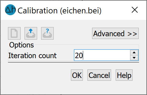
Calibration

After opening „Advanced“ further settings can be made:

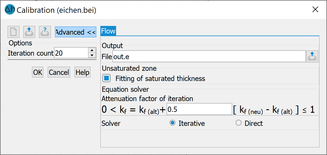
Advanced settings (2D)

After the calculation run, the isolines interpolated from the measured values can be compared with the isolines resulting from the calculated K-values.

To do this, go to File Create plot Top view/map presentation... and add additional data by clicking the plus button next to our existing “Model data | Initial potential head -> Isoline”. Change the source for the new data to Result data, and select Potential head for the Data.The rest of the setting can be configured as we did with EICH so we can compare the two. Additionally, change the colour to red so that you can distinguish between the two datasets. When the window is closed by clicking OK, the settings for this plot are saved in the batch file "plo.bpl" (preset).

The following plot shows the result of the first calibration:

Target (green) and result potential heads (red) after the 20th iteration

The next step is creating a measurement data difference plot and …