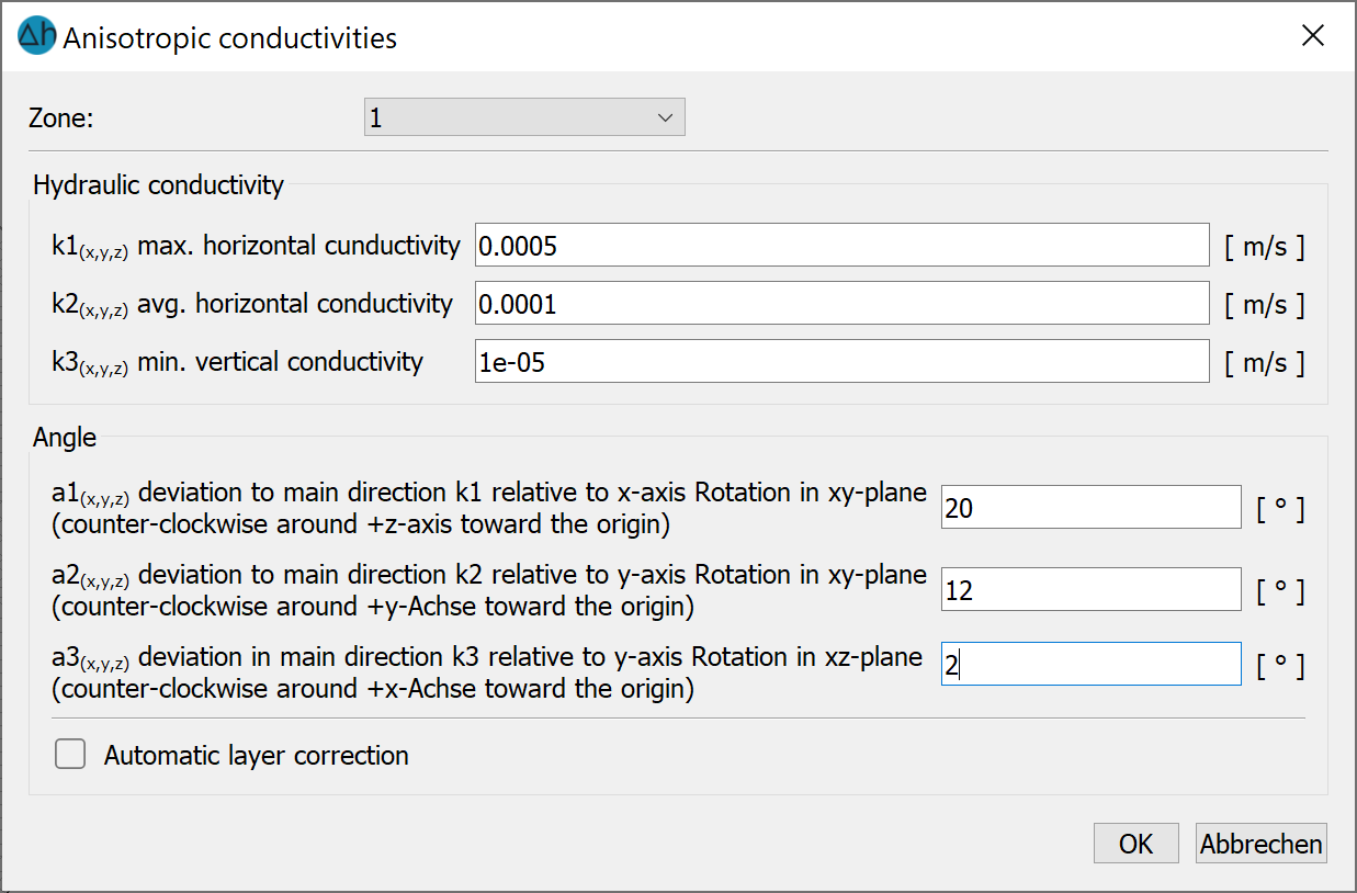
To take anisotropic hydraulic conductivity values into account, a zone (attribute ZONE in the horizontal model, attribute Z-KA in the 3D model) must first be assigned to the elements with the same anisotropy (Attributes Assign Direct...). The individual zones can then be assigned the corresponding K-values and associated angles via the following input window (3D model):

 

 

The following entries are required in the horizontal model:

 

 

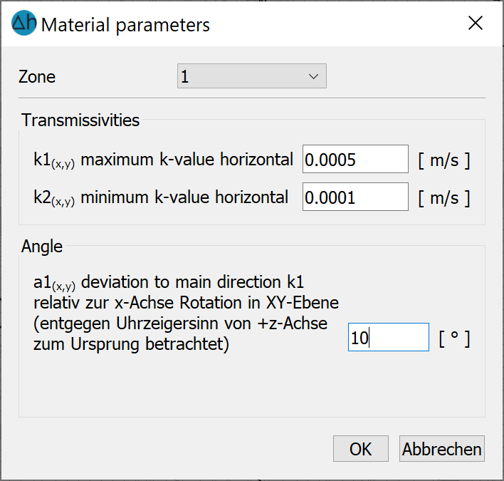
K-values

At this point, anisotropic K-values can be assigned according to their spatial direction.

In the 3D model, the entered K-values K1, K2, K3 together with the angles A1, A2 and A3 are automatically stored zone by zone at the end of the *.3d file of the model after confirming with OK and saving the model. The attribute Z-KA is automatically assigned in the lower layers if it is not assigned there.

In the horizontal model, the provided K-values for K1 and K2 as well as the angle A1 are automatically saved zone by zone in the *.net file under the attribute MATE.

 

Angles

In addition to the direction-dependent K-values, the angles A1 (horizontal and 3D model), A2 and A3 (3D model only) can be defined for a K-value ellipsoid that deviates from the Cartesian coordinate system.

Taking these angles into account, the K-values are corrected according to the following general rotational algorithm:

 

k_korr = H* k_orig* H^T

with:

k_korr = tensor of the (layer-)corrected k-values

k_orig = tensor of the K-values of the model files

H = Rotation matrix with the angles a1, a2, a3

H^T = transposed rotation matrix

 

Angle A1: Counterclockwise rotation in the X-Y plane as viewed from the X-axis.

Angle A2: Rotation in the new X-Z plane in anti-clockwise direction as seen from the new X-axis Angle Angle A3: Rotation in the new Y-Z plane in anti-clockwise direction as seen from the new Y-axis)

 

 

Automatic layer correction (3D only)

In general, the hydraulic conductivity values defined in SPRING (attribute KWER) apply to isotropic flow conditions, i.e. the resulting flow direction is determined by the pure potential gradient of the aquifer without consideration of the geometric discretisation.

By activating this button, an optional (and automatic) layer correction takes place, in which the K-values are automatically adjusted to the element or layer geometry. As the element geometry usually adapts to the geological stratification of the model area, a geometric correction of the hydraulic conductivity is made without specifying angles.

For the internal calculation, the centre plane between the upper and lower "element surface" is generated and its normal is calculated. The deviations of the normals from the respective coordinate plane result in the angles A1, A2, A3, with which the K-values are corrected according to the general rotation algorithm described above.

If the K-values are to be corrected for ALL layers, it is not necessary to assign the Z-KA attribute. To do this, it is sufficient to insert the following line at the end of the batch file sitra.b:

 

ROTATION KWER

 

The following figure shows the result of the flow calculation with (red potential lines) and without (blue potential lines) consideration of the layer-corrected K-values for all layers:

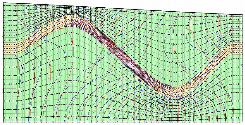
Comparison of the potential lines with (red) and without (blue) layer-corrected K-values for all layers

The yellow layer is impermeable against the green layers by a factor of 100.

 

The yellow layer is 100 times more impermeable than the green layers. The differences in the calculation method are particularly evident where the gradient of the geological layer opposes the horizontal groundwater flow.

If the K-values are only to be adapted to the geological course for selected layers, this is achieved by using zoning with the Z-KA attribute.

To do this, select the relevant zone in the dialogue and activate the "Automatic layer correction" button.

The following figure shows a model in which only layers 9 to 11 were defined as zone 2. The K-values are the same for all layers (horizontal 0.0001, vertical 0.0001), as the corresponding element attributes show:

 

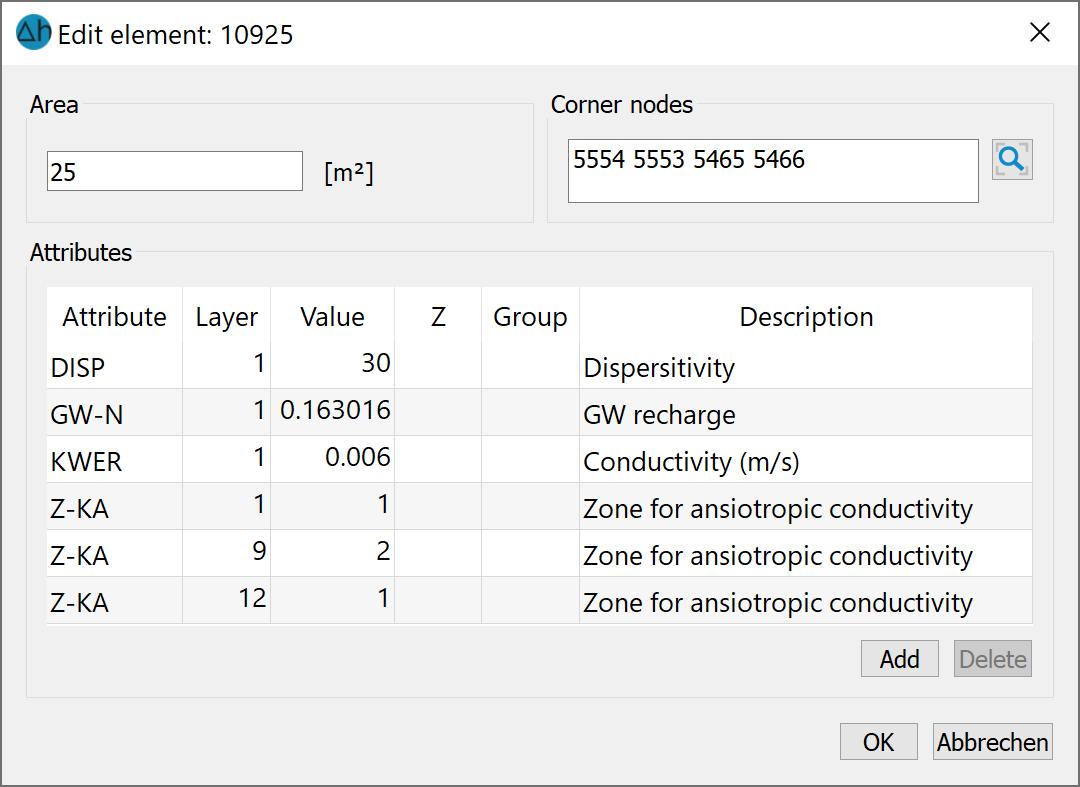
Due to the automatic reallocation, the Z-KA attribute must be reassigned from layer 12 onwards, as zone 2 should only apply to layers 9 to 11.

An automatic layer correction was then carried out for zone 2. The following figure shows the result of the flow calculation:

 

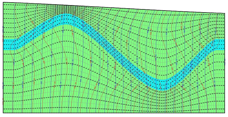
Comparison of the potential lines with (red) and without (blue) layer-corrected K-values in zone 2

Zone 2 comprises layers 9 to 11, which are coloured turquoise in the illustration. Zone 1 is all other layers (green).

 

 

Map