Access via selection in the menu from File Export Schlieren plot

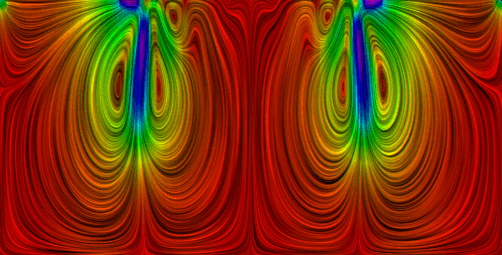
With the FLIC programme (Konrad-Zuse-Centre for Information Technology Berlin), it is possible to display the calculated velocities as "streaks" after a flow calculation. The method used here is called "Line Integral Convolution (LIC)". This visualisation technique provides a much better idea of flow paths than the flow arrows that can be displayed in the plotter. This applies in particular to transient calculations and 3D models, where streamline calculations are sometimes not possible.

 

 

The data export generates the ASCII files required for FLIC.

As the ASCII interface to the FLIC programme is based on raster data, it is necessary to calculate the velocities at the raster points.

FLIC allows the streaks to be coloured either according to the size of the velocities or according to another scalar parameter that is to be defined at all grid points. For this purpose, a result or model data type that is available for all nodes or elements can be specified for colouring the streaks (e.g. colouring the streaks according to concentrations or potential heads). In addition, existing markers are output as possible overlay files (*.mar).

FLIC is called up automatically during data export or can be started manually in the command line:

 

flic cmd=<command file> (*.scr)

 

FLIC then generates a bitmap in jpg format, which can be read with a suitable graphics programme. For 2D horizontal models and horizontal sections of 3D models, the corresponding world file (ending *.jgw) is also generated with the necessary georeferencing information. The commands permitted for FLIC are listed below, which can also be entered directly in the command line.

 

cmd=<filename> read more commands from a file

field=circle use a circular vector field

field=spiral use a spiral-type vector field (default)

field=<filename> read a vector field from a file

out=<filename> name of the resulting LIC image (required)

size=<nx>x<ny> size of noise input image (default 256x256)

in=bwnoise create black-white noise image

in=colornoise create color noise image

in=<filename> use given image file as input

resize=<nx>x<ny> resize current input image

kernel=box select box filter kernel

kernel=triangle select triangle-shaped filter kernel (default)

kernel=cubic select third-order B-spline filter kernel

length=<n> length of filter kernel in pixels (default=20)

subpix=<n> enable nxn super-sampling to reduce aliasing

contrast=raw no contrast adjustment (default for file input)

contrast=auto contrast adjustment (default for noise input)

enhance=0 disable post-filtering of LIC image (default)

enhance=sharpen compute directional derivative of LIC image

enhance=emboss,<a> apply emboss filter, angle arg is optional

integrator=euler use Euler method for field integration

integrator=rk43 use adaptive Runge-Kutta integrator

interpol=const nearest-neighbour interpolation of input image

interpol=bilinear bilinear interpolation of input input (default)

colorfield=dir color denotes vector orientation (fixed colormap)

colorfield=mag compute color from vector field magnitude

colorfield=<file> compute color from scalar field stored in file

colormap=hueramp use hueramp for pseudocoloring

colormap=hotiron use rot-yellow-white colormap

colormap=<file> read colormap from file (icol format)

colorrange=auto colormap min max adapted to colorfield (default)

colorrange=min,max specifies colormap min max values

overlay=<file> render graphics on top of output image

verbose=0|1 enable verbose mode (default is off)

 

Input parameters