The first calibration provides a good starting point for the K-values. These are obtained via Attributes Import model data/result data... and can be copied into the model file by specifying a target.

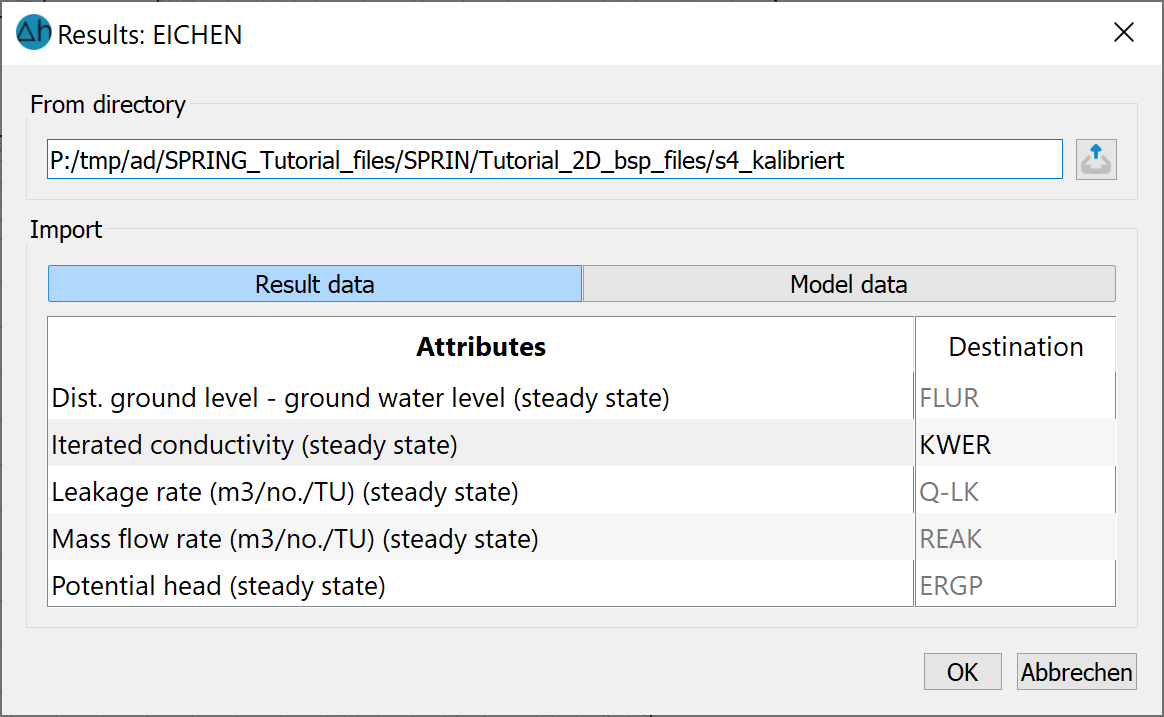
Reading in results data

Keep in mind that when we select the KWER attribute identifier as the target, the existing K-values are overwritten. To avoid large jumps in the K-values in neighbouring elements, the new K-values must be smoothed as follows:

Attributes Compute Smoothing…: In the resulting window select KWER as the attribute, set the weighting factor to 0.5, and keep the weighting type as "linear". Since attributes have been changed, save the model file. The model must then be checked (Calculation Model checking…), a flow calculation (Calculation Steady state flow) with 5 iterations and the GEONEU module ( Advanced settings) is calculated and a new plot is created with the previously saved "plo.bpl" batch file. The result is shown in the following image:

Isolines with difference plot after smoothing the K-values

The maximum deviation at the measuring points is 0.50 m, the average is 0.09 m. The course of the isolines in the upper reaches of the stream indicates infiltration of the stream water into the groundwater. The isoline "17.75 (red)" forms a peak in the direction of flow when it "crosses" the stream.

As this does not correspond to the actual conditions here (stream bed is probably dry), the parameter MXKI = 0.0 is assigned to the last 14 nodes, i.e. infiltration is prevented (Attributes Assign Direct...).

After running the model check, a steady-state flow calculation and plotting, the following picture emerges:

Isolines with difference plot after introduction of MXKI at 14 nodes

The infiltration in the upper reaches of the stream has been eliminated. The course of the isolines is more plausible, but the average deviation of the measuring points has worsened. The maximum deviation is now 0.39 m and the mean at 0.17 m. There seems to be too little water in a large part of the model!

It makes sense to start a calibration again with the parameters changed up to this point. The result is the following image:

Isolines with difference plot after recalibration

Finally, the iterated K-values are transferred to the model file, smoothed and a new flow calculation is performed. The current mesh file "s4_calibrated" results in this image (diagram: .../Tutorial_bsp_files/Tutorial_2D_bsp_files/s4_calibrated.zip):

Isolines with difference plot of the calibrated model

The deviations at the measuring points are a maximum of 0.41 m and 0.08 m on average. This is considered to be sufficiently accurate for the example model.

The distribution of hydraulic conductivities now looks as follows:

Distribution of the calibrated hydraulic conductivities

The hydraulic conductivities were displayed (via View Show attributes Attributes… or by clicking on the Isolines/area plots/values toolbar item) in the interval 1.0e-06 to 0.002 within 10 value ranges. By opening the project manager, the layer list appears in a new window, in which the arrangement of the individual layers can be changed using drag & drop (note: "Top" in the layer list corresponds to the very front, "Bottom" in the layer list corresponds to the very back). Click on the arrow next to the “Contour areas KWER” to display the legend of the corresponding layer.

Legend of the hydraulic conductivity values [m/s]

A step-by-step model calibration can be carried out as described, but it always requires the user to have knowledge of the local conditions and cannot be carried out in a standardised manner. In addition, a plausibility check of the (iterated) parameters should be carried out at the end of a calibration.

General notes on calibration