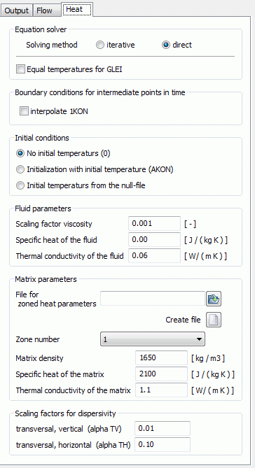
After calling the dialog window "Heat" the following input window appears.

Equation solver
For solving the equation system there are an iterative PCG solver and a direct Cholesky solver. For meshes of about 500 nodes or more, you should always choose the iterative one, because it is much faster. The error due to the iterative solution is always much smaller (less than 3%) than the other errors (e.g. measurement error). This can be verified with the help of the mass balance printed to the output file.
Equal temperatures for GLEI
This determines whether at nodes with the attribute GLEI also the equal temperatures should be calculated.
Boundary conditions at intermediate point in time
If the calculation is done with a fixed time step size or diminished time steps of the transient input file, it is possible at the intermediate time steps, which are not regulated by the transient input file to interpolate transient boundary conditions for the temperatures.
Initial conditions
Here is defined with which initial temperatures the transient heat transport calculation is started:

No initial temperatures: The iteration is started with initial temperatures = 0.0 (not recommended).

Using initial temperatures: The initial temperatures of the model file (attribute AKON) are used.

The transient calculation can be continued, if the corresponding null-file from the previous calculation exists (warm start). If the user wants to continue the actual calculation, the program has to create the corresponding file called out66. This is specified in the choice of output parameters (Save for continuing (out66) ).
Fluid parameters
The scaling factor viscosity (η0) scales the underlying formula for the calculation of the dynamic viscosity as a function of the model species:

by:

For vertical- or 3D models is η0 = 1.0 [-] (default), because in the calculation of these model types, the pressure equation is used. In horizontal models is η0 = 1000.0 [-], because in the calculation of this model type, the potential equation is used.
The specific heat capacity of the fluids in [J/(kg K)] has to be entered.
The heat conductivity of the fluid in [W/(m K)] has to be entered.
Matrix parameters
If the zoning attribute Z-KD is available in the model file, the associated file with the zoning data can be selected for the matrix parameters.
The density of the matrix in [kg/m³] has to be entered.
The specific heat capacity of the matrix in [J/(kg K)] has to be entered.
The heat conductivity of the matrix in [W/(m K)] has to be entered.
Creating a new file with zoning data is explained in the chapter "Structure of the zoning files".
Saving the dialogue above results in the following entry in the file with the zoned heat parameters:
Zone nr spec. heat capacity (matrix) heat conductivity (matrix) density (matrix)
1 2100 1.1 1650 #Zone number CS SIGMAS RHOS
Dispersivities
Defining transversal-horizontal (αTH) and transversal-vertical (αTV) dispersivities [m].
The scale refers to the longitudinal dispersivity, which is defined in the model file using the attribute DISP.
 Results of the heat transport calculation
