
PL3D
The command PL3D creates a 3D plot, when the user writes himself the corresponding batch file. Below are several examples of such files.
Input (separated by a blank or a tab):
1st line: direction of view (0 degree = W, 90 degree = S, 180 degree = O, 270 degree = N), point of view (> 0 from top, < 0 from bottom), scaling factor in z-direction and the focus (> 0, parallel projection for focus = infinite)
2nd line: nx, ny (grid division: number of intervals in x and y direction)
3rd line: data identification number for the basic level of the 3D representation, time step and layer number
4th line: grid level (≤ data minimum), colour number, line thickness, line type
5th line: data identification number for grid plot, time step, layer number:
6th line: Add equal-value lines to the grid? Data identification number, time step, layer number
7th line: Colour number, line thickness, line type
Examples:
To create 3D plot with the following PL3D blocks, the corresponding *.bpl file has to contain the two lines
DATE ## file name of the plot file
bild.plx
at the beginning of the file and the line
# ---> Plot Ende!
at the end of the file.

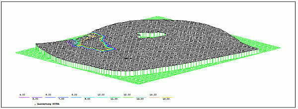
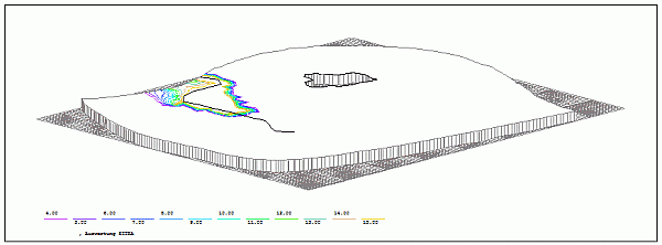
3D plot with a monochrome grid at the level of the potential head and coloured equal-value lines for the concentration:
PL3D # 3D-plot
135. 15. 10. 1.e+6 #direction of sight: SW, angle of direction, elevation factor z,focus
100 100 # 100x100 raster
201 # Raster from height of potential heads
0. 3 0.25 1 # Raster level at potential=0. in colour 3
-1 # monocoloured raster
1 0.25 1 # colour 1, line width, line type ...
203 # Isolines for concentartions (203),
0 0.25 1 # different colours! Colour to begin with=0
2 # Isolines
4. 16. 1. # from, to distance
1 0.5 1 # Markers in colour 1, line width 0.5, line type 1
|
|
|

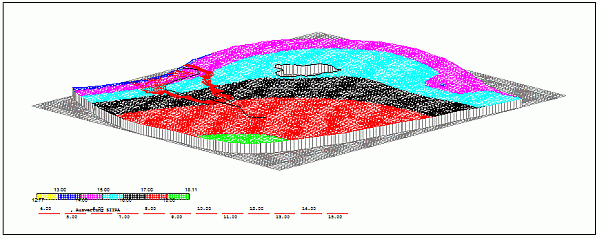
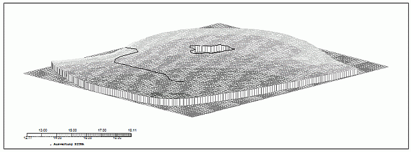
3D plot at the level of the potential head with a multi-coloured grid for the potential head and monochrome equal-value lines for the concentration:
PL3D # 3D-plot
135. 15. 10. 1.e+6 # direction of sight: SW, angle of direction, elevation factor z,focus
100 100 # 100x100 raster
201 # Raster from height of potential heads
0. 8 0.25 1 # Raster level at potential=0. in colour 8
201 # Raster for potentials
4 0.25 1 # multi-coloured raster, starting colour 4 ...
2 # Raster colour interval for potentials (201)
13. 18. 1. # from, to, distance
-203 # Isolines for concentrations (203),
2 0.25 1 # monochrome (colour 2)
2 # Isolines
4. 16. 1. # from, to distance
1 0.5 1 # Markers in colour 1, line width 0.5, line type 1
|
|
|

3D plot (without grid) with coloured equal-value lines for the concentration at the level of the potential head:
PL3D # 3D-plot
135. 15. 10. 1.e+6 #direction of sight: SW, angle of direction, elevation factor z,focus
100 100 # 100x100 raster
201 # Raster from height of potential heads
0. 8 0.25 1 # Raster level at potential=0. in colour 8
0 # no raster
203 # Isolines for concentrations (203),
0 0.25 1 # different colours! Starting colour=0
2 # Isolines
4. 16. 1. # from, to, distance
1 0.5 1 # Markers in colour 1, line width 0.5
|
|
|

3D plot at the level of the potential head with a multi-coloured grid for the potential head, without additional equal-value lines:
PL3D # 3D-plot
135. 15. 10. 1.e+6 # direction of sight: SW, angle of direction, elevation factor z,focus
100 100 # 100x100 raster
201 # Raster from height of potential heads
0. 8 0.25 1 # Raster level at potential=0. in colour 8
201 # Raster for potentials
-1 0.25 1 # multi-coloured raster, in gray (starting colour -1 ...)
2 # Raster colour interval for potentials (201)
13. 18. 1. # from, to distance
0 # no isolines
1 0.5 1 # Markers in colour 1, line width 0.5
|
|
|

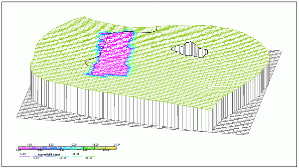
3D plot at the level of the potential head after 10 days with a multi-coloured grid for the concentrations and multi-coloured equal-value lines for the concentrations:
PL3D ## 3d-Schaubild
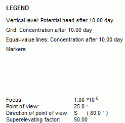
80.0 25.0 50.0 1000000.0 # direction of sight: SW, angle of direction, elevation factor z,focus
60 60 # 60x60 raster
301 10 1 0 # Height: Potentials (time step 10), layer 1, Index
1.00 8 0.25 1 # Raster level at potential=1., colour 8, ...
303 10 1 # multi-coloured raster: conc. (time step 10), layer 1
0 0.25 1 # Starting colour 0, line width, line type
3 8 # single values -> number of values
1.00000 3.00000 5.00 8.0000 10.0000 #
12.0000 15.00000 20.00000 #
303 10 1 # multicoloured isolines: conc. (ts 10), layer 1
0 0.30 1 # starting colour, line width, line type
3 6 # single values -> number of values
1.00000 3.00000 5.00000 10.00000 12.00000 #
20.00000 #
1 0.25 1 # Markers in colour 1, line width 0.25
|
|
|

 1D fracture data