After calling up the "Heat" dialogue window, the following input window for the heat parameters appears.

 

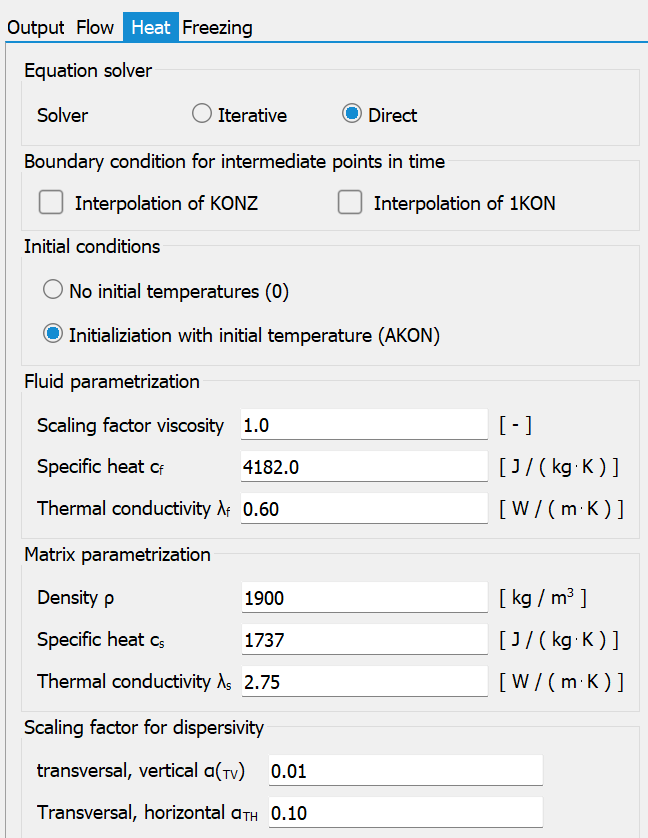
Equation solver

Either the iterative PCG solver or the direct Cholesky equation solver can be selected as the equation solver. Due to its advantages in terms of computing time and memory space, the iterative equation solver is recommended from approx. 500 nodes. In contrast to the direct method, the solution is not calculated exactly, but the error is usually negligible. An accuracy check can be carried out using the mass balance specified in the output file.

 

Equal temperatures for GLEI

Here you can specify whether the same temperatures should also be calculated at nodes with the GLEI attribute.

 

Boundary conditions for intermediate point in time

If the calculation is performed with a fixed time step size or with reduced time steps of the transient input file, it is possible to interpolate the transient boundary conditions for the temperatures for the intermediate time steps that are not defined in the transient input file! In principle, the same explanations that already apply to the transient flow calculation apply.

 

Initial conditions

The initial temperatures with which the transient heat transfer calculation is started are defined here:

• No initial temperatures: The iteration is started with initial temperatures = 0.0 (not recommended!).

• Initialisation with initial temperature (AKON): The initial temperatures defined in the model file via AKON are used here.

• If a transient calculation has already been carried out, this can be continued with the result temperatures saved in the null-file. This is specified when selecting the output parameters (Save for continuation (out66)).

 

Fluid parametrisation

The viscosity scaling factor (η₀) scales the formula for the dynamic viscosity on which the calculation is based depending on the model type:

 

through:

 

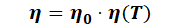
For vertical or 3D models, enter η₀ = 1.0 [-] (default setting), as the pressure equation is used in the calculation of these model types.

For horizontal models, enter η₀ = 1000.0 [-], as the potential equation is used in the calculation of this type of model.

Enter the specific heat capacity of the fluid in [J/(kg K)]. The thermal conductivity of the fluid must be entered in [W/(m K)].

 

Matrix parametrisation

If the zoning attribute Z-KD is present in the model file, the associated file with the zoned data (p. 44) for the matrix parameters can be selected here.

The density of the matrix must be entered in [kg/m³].

Enter the specific heat capacity of the matrix in [J/(kg K)]. The thermal conductivity of the matrix must be entered in [W/(m K)].

The creation of a new zoning file is explained in the chapter "Structure of the zoning files".

The dialogue shown above results in the following entry in the file with the zoned heat parameters:

 

Zone nr spec. heat capacity (matrix) heat conductivity (matrix) density (matrix)

1 2100 1.1 1650 #Zone number CS SIGMAS RHOS

 

Scaling factor for dispersivity

Specify the scaling factors for the transversal-horizontal (α_TH) and transversal-vertical (α_TV) dispersivities [m].

The scaling refers to the longitudinal dispersivity, which is defined in the model file by the DISP attribute.

 

Freezing