After clicking the "Flow" tab option, the following input window appears (depending on the data type available in the mesh file:
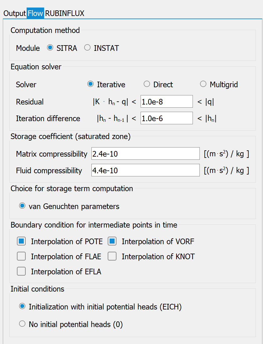
Calculation method
The two computation modules SITRA and INSTAT are available (the XTRA module will be available in the near future). The default setting is a calculation with the SITRA module. The INSTAT module must be selected for a horizontal model with a three-dimensional sub-area.
Equation solver and termination criteria
The procedure for the solution methods and the termination criteria have already been described in the calculation of the steady state flow.
Storage coefficient
The following parameters can be changed here:
The specific storage coefficient for horizontal models (confined aquifer) or the fluid and matrix compressibility for 3D models (saturated/unsaturated calculation).
Storage term calculation
The storage term calculation is based on the van Genuchten parameters.
Boundary conditions for intermediate points in time
If the calculation is performed with a fixed time step size or with reduced time steps of the transient input file, it is possible to interpolate the transient boundary conditions for the intermediate time steps that are not defined in the transient input file.
In principle, the following is assumed:
Transient subsidence is always interpolated linearly!
If a point in time is listed in the transient input file (even without data), the boundary conditions (exception BERG) for this point in time are not interpolated, i.e. only the data that are listed as data blocks below are changed. All other boundary conditions remain those of the previous time step! The following examples serve to illustrate this:
Example 1:
The model file states: POTE 10.0 1,...., i.e. node 1 has a fixed potential head of 10 m above sea level. The transient input file reads:
ZEITEINHEIT ZEIT TAG
ZEIT (first date)
2.0
POTE
1 12.0
i.e. the fixed potential head of node 1 is set to 12 m above sea level in the 2nd time step.
In the case of a transient calculation with a time step width of 1-day, different behaviour result depending on the specification for the interpolation of the boundary conditions for intermediate times for the transient boundary condition:
a) with interpolation of the boundary conditions:
10.0 for the 0th time step (is not actually analysed, input in model file)
11.0 for the 1st time step (i.e. on the 1st day)
12.0 for the 2nd time step (i.e. on the 2nd day)
b) without interpolation of the boundary conditions:
10.0 for the 0th time step (is not actually analysed, input in model file)
10.0 for the 1st time step (i.e. on the 1st day)
12.0 for the 2nd time step (i.e. on the 2nd day)
Example 2:
The model file again contains: POTE 10.0 1,…
The transient input file contains:
ZEITEINHEIT ZEIT TAG
ZEIT (first time step)
1.0 (without data)
ZEIT (2nd time step)
2.0
POTE
1 12.0
i.e. the fixed potential head of node 1 is set to 12 m NN in the 2nd time step.
The boundary conditions at node 1 do not change on day 1. The fixed potential head is also set on day 1 to 10.0 m above sea level. A desired change must be specified explicitly! The fixed potential heads in node 1 are as follows
When entering 1-day increments as a fixed time increment or when calculating with the time increments of the transient input file (also daily increments) with and without interpolation of the boundary conditions:
0 for the 0th time step (is not actually analysed, input in model file)
0 for the 1st time step (i.e. on the 1st day)
0 for the 2nd time step (i.e. on the 2nd day)
When entering 1/2 day increments as a fixed time increment or when calculating with 1/2 time increments of the transient input file (also 1/2 day increments):
a) with interpolation of the boundary conditions:
0 for the 0th time step (is not actually analysed, input in model file)
0 for the 1st time step (i.e. on 0.5 day)
0 for the 2nd time step (i.e. on the 1st day)
0 for the 3rd time step (i.e. on day 1.5)
0 for the 4th time step (i.e. on the 2nd day)
b) without interpolation of the boundary conditions:
0 for the 0th time step (is not actually analysed, input in model file)
0 for the 1st time step (i.e. on 0.5 day)
0 for the 2nd time step (i.e. on the 1st day)
0 for the 3rd time step (i.e. on day 1.5)
0 for the 4th time step (i.e. on the 2nd day)
Please note: Transient boundary conditions are always treated explicitly. This means that the boundary conditions of time tn are used to calculate the state for time tn+1.
Initial conditions
The initial potential heads with which the transient calculation is started are defined here.
Using the calibration potential heads as initial potential heads: The result potential heads of the steady state flow calculated after calibration are used as initial potential heads. To do this, the result potential heads must be copied to the identifier EICH in SPRING via Attributes
 Import Model data/result data Potential head.....
If a transient calculation has already been carried out, this can be continued with the result potential heads saved in the null-file. This is defined when selecting the output parameters (Save for continuation (out66)).
No initial potential heads: The iteration is started with starting potential heads = 0.0.
Stand: 11.06.2025 | 