Call by Attributes Compute Groundwater recharge RUBINFLUX Create input_id (grid-based)...

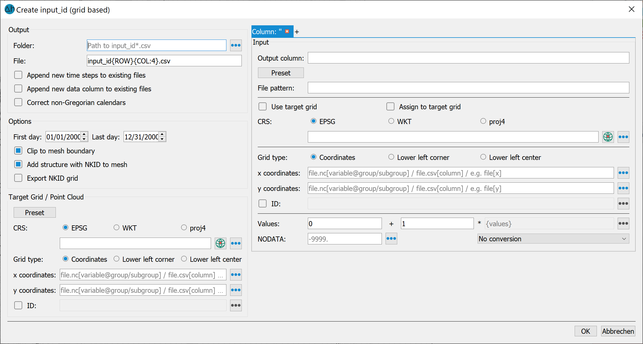
The following input window appears:

 

Remark:

The right side of the dialog window is used for defining the input data (climate time series, e.g. from HYRAS or other weather/climate grid data).

The left side of the dialogue describes the output mechanisms for generating the input_idName.csv files required for calculating the groundwater recharge rates in SPRING.

Entries in curly brackets can be edited by the user, or the cells can be automatically filled by the program. They describe a form for reading data.

 

Input data (right side)

The procedure is described using HYRAS precipitation grids in combination with EVAPO-P grids and HYRAS temperature grids (all from the DWD). A separate tab is created in the upper right corner for each type of data to be imported. Their order corresponds to the column order in the output files. The order can be changed via drag and drop.

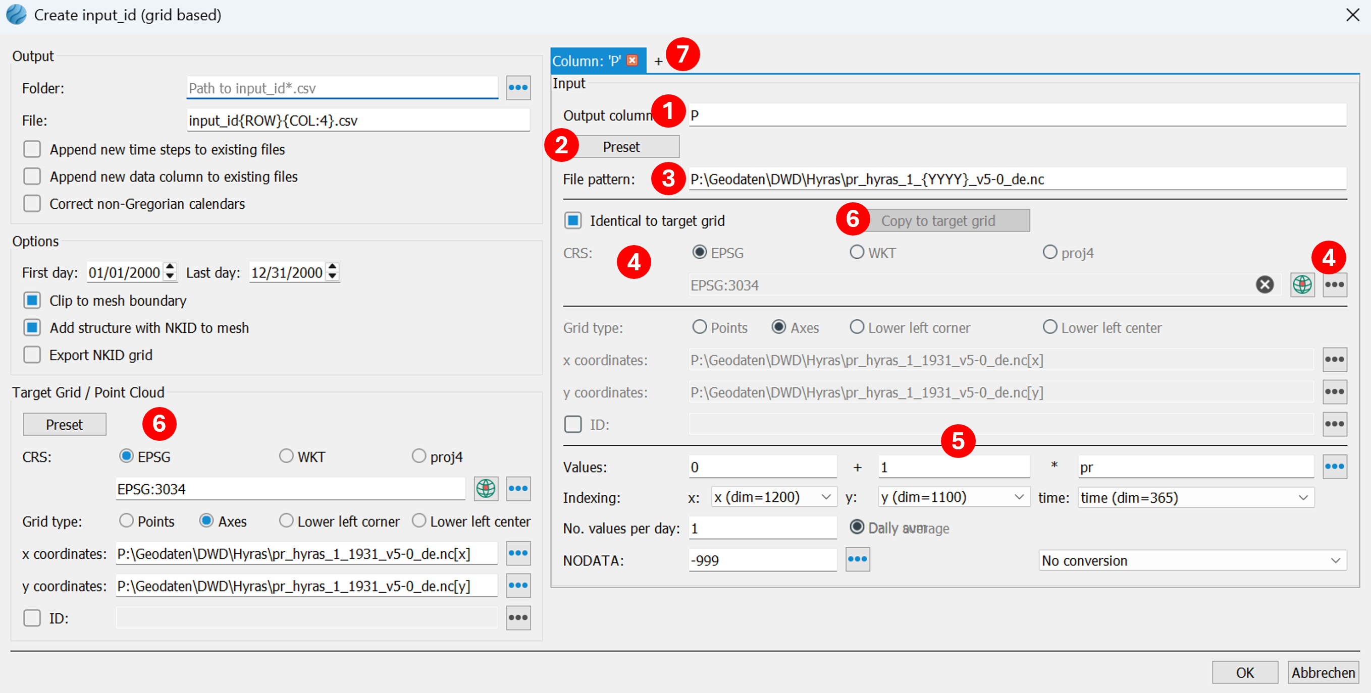
(1) The first column for the combination shown should always be the precipitation P; enter P in the target column name field.

 

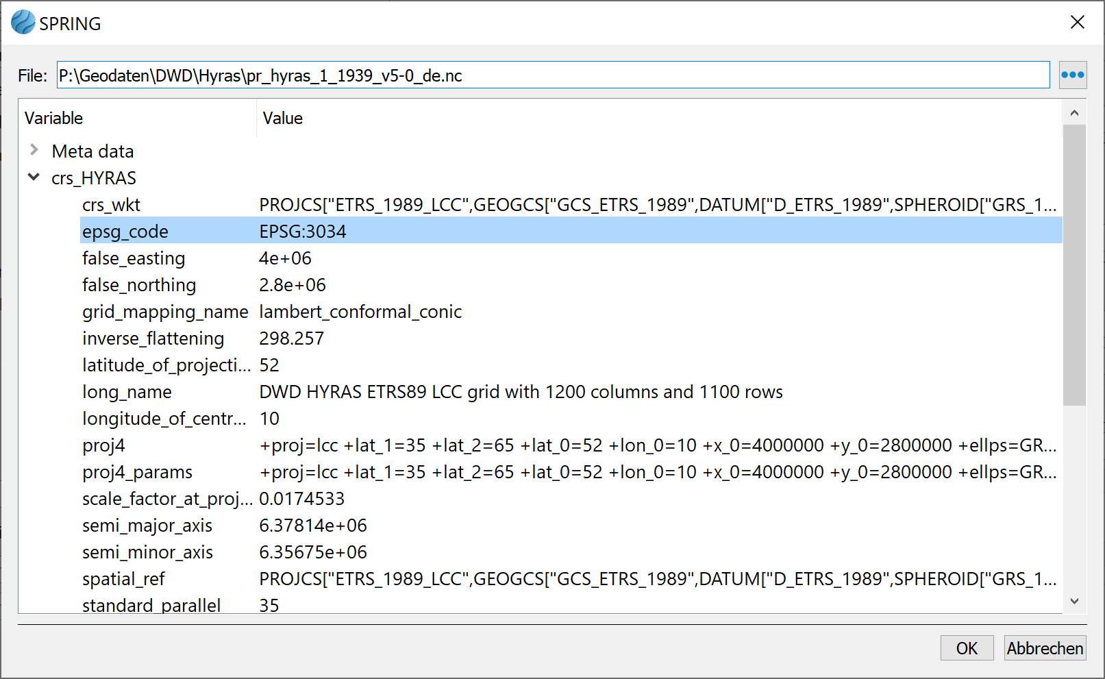
(2) Then, using the Preset button, navigate to a *.nc file (NETCDF format), e.g., pr_hyras_1_1931_v5-0_de.nc, containing HYRAS precipitation data, and select it. Since the NETCDF format contains extensive metadata, additional fields on the right will be automatically populated.

(3) Now the entered file template must be generalized so that the program can find the files for all desired years. HYRAS data is stored as year data in separate files. The year in the file template is manually changed to {YYYY}.

Example:

File template before:

..\ Hyras\pr_hyras_1_1931_v5-0_de.nc

File template afterwards (generalized):

..\ Hyras\pr_hyras_1_{YYYY}_v5-0_de.nc

Note: Time series data for climate projections sometimes come in raster files containing 5-year periods. The input in the file template must then be adjusted as follows:

• {YYYY%5} means rounded to the nearest "remainder 5", e.g. 2020, 2025, 2030, ...

• {YYYY%5+1} first calculates "remainder 5" and then adds 1., e.g. 2021, 2026, 2031, ...

• This method only works for years and only if 4 digits are used for the year.

 

(4) The coordinate reference system (CRS) of the HYRAS data is filled in by pressing(only works with NETCDF files) and select the line epsg_code there. Alternatively, it can be selected manually with

 

(5) All other parameters required for correctly reading the HYRAS data have already been automatically populated. Spatial reference is established via the grid type (axes) and the definition of the X and Y coordinates. No correction factors are necessary for the HYRAS values. The NODATA value is also read from the metadata.

 

(6) The time series use different grid sizes. The HYRAS precipitation data are in a 1x1 km grid, while the evapotranspiration data are in a 5x5 km grid. It is recommended to use the finer HYRAS grid as the target grid for output to SPRING. This happens automatically via the "Copy to target grid" button. This automatically fills in the "Target grid/point cloud" area on the left side of the input mask and activates the "Identical to target grid" checkbox.

The input form now looks like this:

(7) The second column will contain the potential evapotranspiration from grass. A new column is created using the "+" button. The target column name is ET0.

 

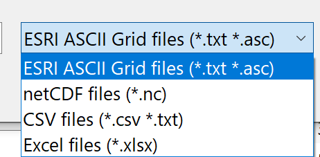
(8) Use the Preset button to navigate to and select a *.asc file, e.g., grids_germany_daily_evapo_p_19910101.asc, containing EVAPO-P data. The ESRI ASCII grid format also includes metadata, and additional fields on the right-hand side will be automatically populated.

 

(9) Now the entered file template must be generalized so that the program can find the files for all the desired days. EVAPO-P data is stored as daily data in separate files and sorted by year and month in subfolders. Therefore, all date information in the file path and file name must be generalized accordingly.

File template before:

..\grids_germany_daily_evapo_p_1991\grids_germany_daily_evapo_p_199101\grids_germany_daily_evapo_p_19910101.asc

File template afterwards (generalized):

..\grids_germany_daily_evapo_p_{YYYY}\grids_germany_daily_evapo_p_{YYYY}{MM}\grids_germany_daily_evapo_p_{YYYY}{MM}{DD}.asc

 

(10) The coordinate reference system (CRS) of the EVAPO-P data is filled in by pressing and manually selecting EPSG: 31467.

 

(11) The parameters for the grid type have already been automatically set: bottom left corner, corresponding coordinates, number of columns and rows, and cell size. EVAPO-P values are in centimeters and must therefore be multiplied by the correction factor 0.1. The NODATA value is read from the metadata.

 

 

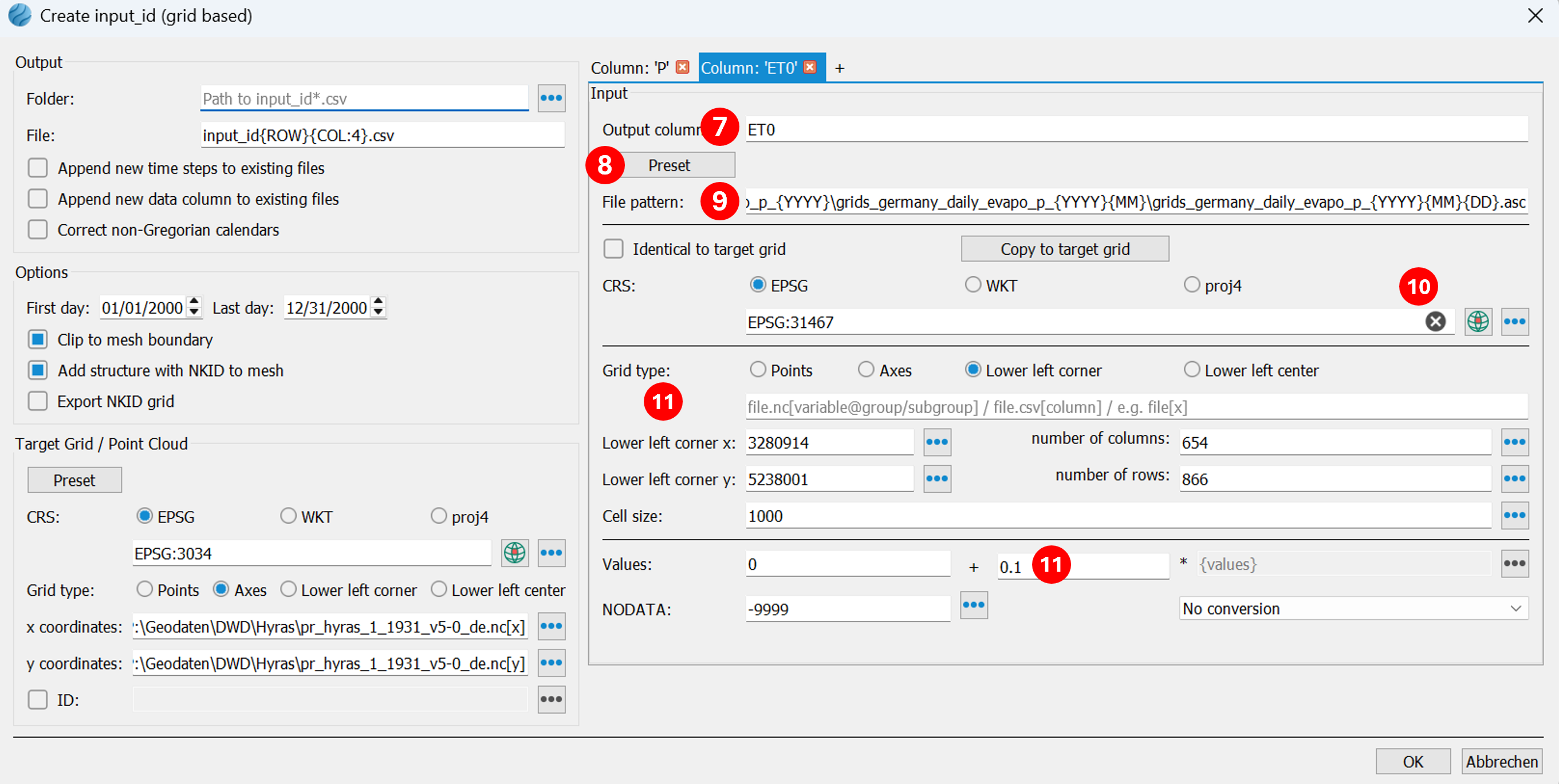
(12) Since the finer HYRAS raster is to be used as the target raster, no target raster specification needs to be entered in the ET0 tab. The coarser EVAPO-P raster data will be automatically converted to the finer raster during output.

(13) The third column contains the average air temperature. This is needed if snowfall is to be considered in the calculation of snow formation. A new column is created using the "+" button. The target column name is T.

 

(14) Then, using the Preset button, navigate to a *.nc file (NETCDF format), e.g., tas_hyras_1_1970_v6-1_de.nc, containing HYRAS temperature data and select it. Since the NETCDF format contains extensive metadata, additional fields on the right will be automatically preset.

 

(15) Now the entered file template must be generalized so that the program can find the files for all desired years. HYRAS data is stored as year data in separate files. The year in the file template is manually changed to {YYYY}.

Example:

File template before:

..\Hyras\Temperatur\tas_hyras_1_1970_v6-1_de.nc

 

File template afterwards (generalized:

..\Hyras\Temperatur\tas_hyras_1_{YYYY}_v6-1_de.nc

 

(16) The coordinate reference system (CRS) of the HYRAS data is filled in by pressing(only works with NETCDF files) and select the line epsg_code there. Alternatively, it can be selected manually with

 

(17) All other parameters required for correctly reading the HYRAS data have already been automatically configured. Spatial reference is established via the grid type axes and the definition of the X and Y coordinates. Temperature values must be multiplied by a correction factor of 0.1. The NODATA value is also read from the metadata.

 

 

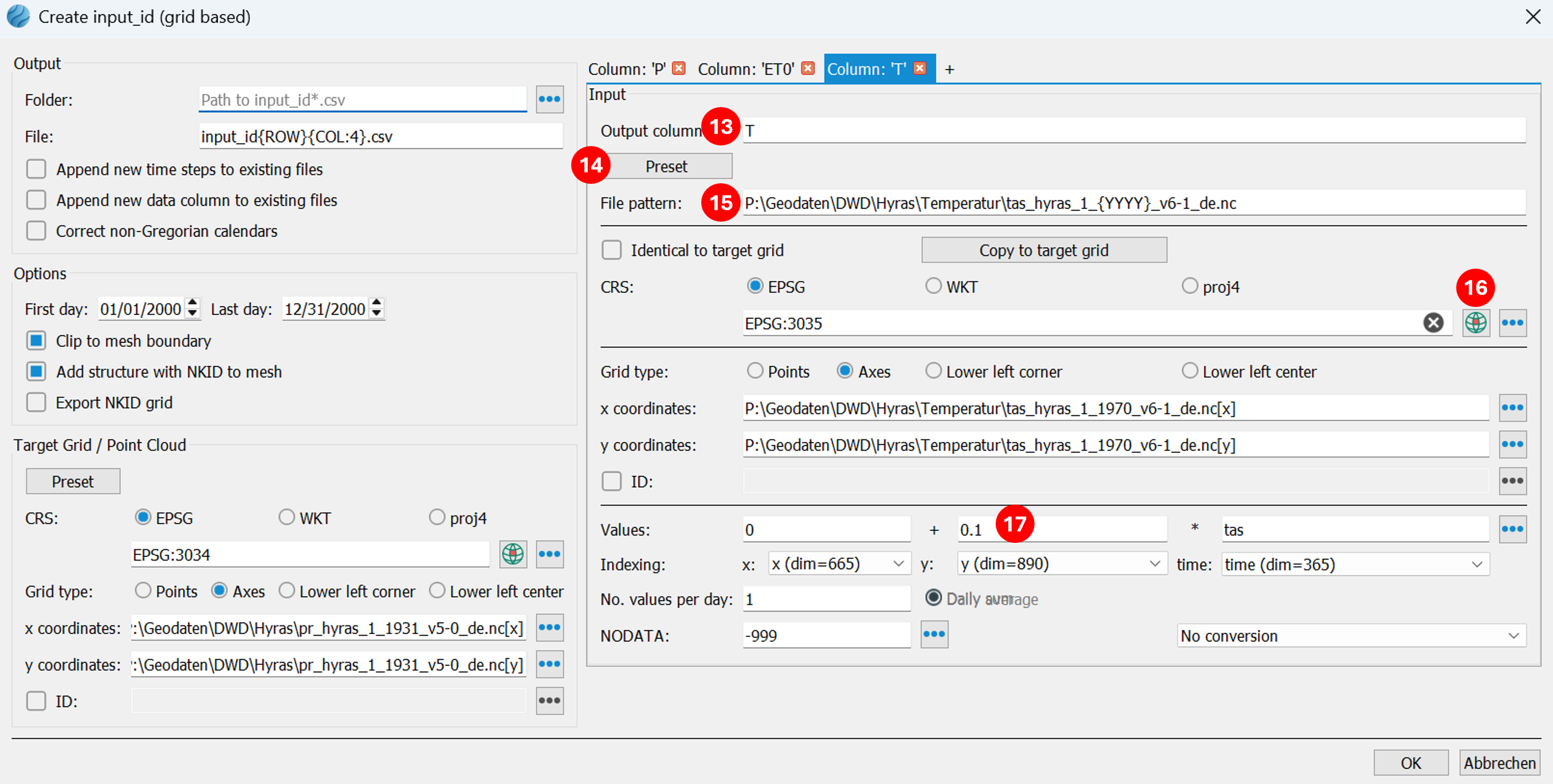
(18) The HYRAS temperature grid is available in 5x5km grids. Since the finer HYRAS precipitation grid is to be used as the target grid, no target grid setting needs to be entered in the T tab. The coarser temperature grid data will be automatically converted to the finer grid during output.

 

Output data (left side)

Finally, the settings for the output files for SPRING are configured on the left side of the input mask.

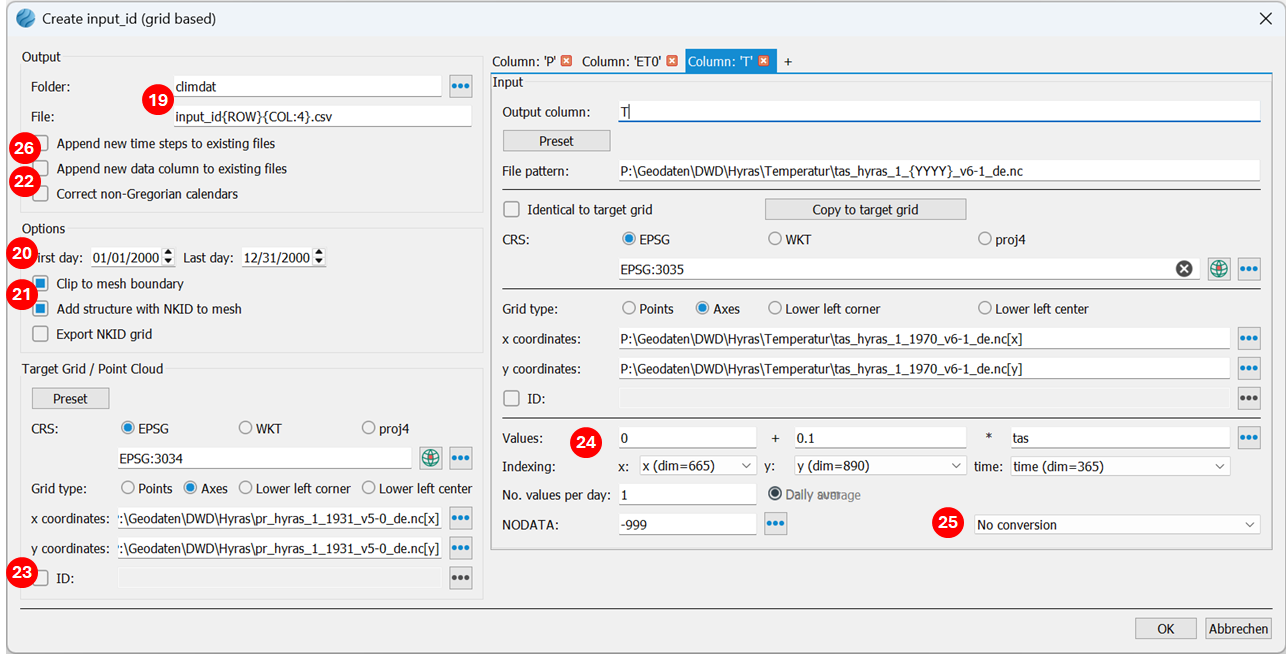
(19) A folder is specified where the input_idNr.csv files will be written. This folder is initially empty in case entirely new input_idNr.csv files are to be created. The file name is automatically generated from the row and column number of the grid. This number also corresponds to the NKID attribute, which is later assigned to each network element for linking purposes.

 

(20) The date range for the analysis must be specified. It should be ensured beforehand that the corresponding time series grids are available for this period.

 

(21) By default, the grids are selected based on the model's mesh boundary (function: Clipping with mesh boundary). Additionally, a structure is generated that allows for easy assignment of the NKID attribute (function: Add structure with NKID to mesh). This structure can also be exported as a separate file (function: Export NKID grid).

The finished input form looks like this:

 

Special functions

(22) The "Correct non-Gregorian calendars" option is activated when time series data are in non-Gregorian calendar formats (without leap years, 30-day months, etc.). Activating the checkbox inserts the missing days (averaging the dates) or removes extra days (e.g., February 30).

(23) If the user wants to assign their own NKID numbers, they can specify a custom file containing these individual numbers by selecting the ID: checkbox. In the output file name field, {ID} must then be used instead of {ROW}{COL:4}.

(24) If, for example, logger data of precipitation with hourly values is available, it is determined here how daily values are calculated, i.e., summed (e.g., for precipitation) or averaged (e.g., temperature).

(25) Here, for time series where the parameter sunshine duration changes to global radiation or vice versa, you select which conversion should take place. Normally, no conversion is necessary.

(26) The generated data can be appended to existing time series data, or an additional data column can be added to existing files.

 

Generate input_ids (station-based)