In Gaussian interpolation, an interpolation function z(x, y), which is made up of a linear combination of Gaussian bell functions for the measurement points, is applied to the available measurement values. The evaluation of this function at an interpolation point provides the interpolation value z for that point.

 

Let there be n measuring points (x_i, y_i), i=1,...n, with corresponding measured values z_i.

The Gaussian bell functions (basic functions g_i) for the measured values are rotation surfaces with their axis in the assigned measuring point (x_i, y_i):

 

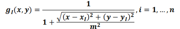
with m: Average of all measuring point distances to each other.

The basic functions are linked linearly to form an area function:

 

z(x, y) = b₁ g₁(x, y) + b₂ g₂(x, y) + ... + b_n g_n(x, y)

 

The coefficients b_j used for the linear combination are unknown and form the shape parameters of the surface function. The determination of the shape parameters results from the requirement that the measured values must lie on the area defined by the area function. A conditional equation results for each measurement point i:

 

z_i = z(x_i, y_i) = b₁ g₁(x_i, y_i) + b₂ g₂(x_i, y_i) + ... + b_n g_n(x_i, y_i)

 

This leads to a symmetrical (n x n) system of equations for the n unknowns b_i , i=1,...n.

After determining the unknowns b_i, the corresponding function value can be calculated for each grid node or for each element centre point with the coordinates x and y by inserting it into the area function z(x,y).

In order to equalise the oscillations in the Gaussian surface function z (x, y), this is also balanced with a further surface function.

 

Z = Z(x, y) = B₁ g₁(x, y) + B₂ g₂(x, y) + ... + B_n g_n(x, y)

 

whose coefficients B_i , i = 1, ... ,n are determined by the condition:

 

Z_i = Z(x_i, y_i) = B₁ g₁(x_i, y_i) + B₂ g₂(x_i, y_i) + ... + B_n g_n(x_i, y_i) = 1 for i=1,..,n.

 

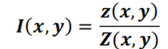
The interpolation value I at a point (x, y) is thus calculated as follows:

 

 

Implementation in SPRING

The implementation in SPRING utilises parallel processing. This makes the algorithm extremely fast and memory-efficient. No further input is required.

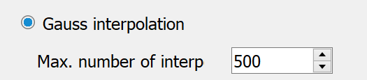
Gaussian input

The maximum number serves as an upper limit for the equation solver.

 

Area interpolation