This menu contains all the representations that are possible for attributes. If a model does not contain one of these items, this item is disabled, i.e. it is gray.
Isolines/area plots/values…
With this menu item contour lines, coloured areas, circular or linear representations of node and element data are created. It establishes a list of all attributes which are assigned to nodes or elements and the user can define which data and how the data is represented. After calling the function, the following input window appears:
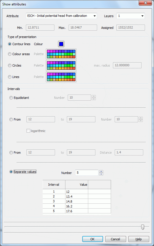
Identifier, details of the attribute
First, the attribute is selected which should be represented. In a 3D model the choice of the layer number is additionally required. If a 2D data type (e.g. ground level) is selected, the layer number is automatically set to 1 and cannot be changed.
The min./max. ranges indicate the minimum and maximum value of this attribute. The next field shows to how many nodes or elements the attribute is assigned in relation to the total number of nodes or elements.
Type of presentation
Possible types are:

Contour lines in a special colour
Colour areas (In case of nodal data, the regions between contour lines are coloured; in case of elemental data, the individual elements are coloured depending on the element value.)
Circle plot, where in each element / at each node a coloured circle is plotted. The radius of the circle depends on the value defined for the element/node. The minimum radius for the circles is 6.0 pixels. In the box max. radius, the maximum radius is defined. To plot all circles with the same radius, set the maximum radius to 6.0 pixels.
Line plot, recommended for attributes that are assigned primarily along a line (e.g. leakage values or equal unknown potential heads along an edge of lake)
Intervals
There are various options:
The equidistant intervals are obtained by a uniform division of the distance between the minimum and the maximum value found. The number of divisions is defined in the box Number.
The type From/to/number defines an interval which is then divided evenly in the chosen number of intervals (text field: number). The defined intervals can be divided logarithmically by activating the check box logarithmic (recommended for K values).
The type from/to/distance is an interval determined by the user.
If separate values are entered, a box appears for the desired interval number and a table in which the interval limits can be defined individually.
If the presentation attributes are chosen, the selected data is stored in a special layer. This layer is listed in the project manager and can be displayed or not. Additionally, the legend of the layer can be displayed by selecting the check box.
Attribute-note…
By using the function Attribute-note, you can display the nodes/elements where for a certain attribute a note is defined, e.g. all VORF nodes with the note ' F' or all FLAE elements with the note ' *'. The following dialogue appears:
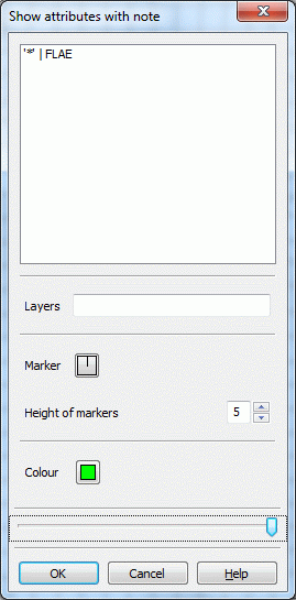
The corresponding menu contains a list of all assigned nodal and elemental attributes from which you can select.
For 3D models, the layer has to be specified. At last, the type, the height and the colour of the marker are determined.
Velocities…
With this menu item it is possible to represent a vector plot of the horizontal velocities defined by the element data types VV_X and VV_Y.
The data has to be imported first from the result data (Attributes  Import data/computation results…). The attribute identifier is pre-set to “VV_X” and “VV_Y”. The following dialogue appears:
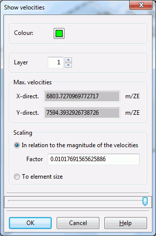
The display colour and, in a 3D model, the layer number have to be selected. The maximum velocities in the x-and y-direction are logged. You can choose between two forms of representation:
The vector length is scaled depending on the velocity. This representation type is equivalent to the representation in the plot generation. The vector length is proportional to the velocity. The arrow is plotted into each element, with the arrowhead at the element centre. For very small velocities, the vectors are plotted with a minimum length.
Alternatively, the vector length is scaled automatically, so that the arrow fits into the element. In this case, the arrow only represents the direction of the velocity, but not its value. The vector length is 80% of the average edge length in the element. The resulting arrow is plotted with its centre at the centre of the element.
Transient…
Transient data are only represented after they were imported via the menu items Special features Transient Import transient input file.
After selecting this menu item the following input window appears:
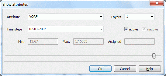
The attributes of the transient input file are shown. Depending on the attribute and the time step the existing minimum and maximum values and the number of assigned nodes or elements are displayed. In a 3D model, the desired layer can be selected.
By selecting the check boxes active/inactive you can distinguish between nodes or elements which are active or inactive. Active means e.g. for the attribute POTE, that at this time step the potential at this node is kept on the entered value. Inactive is a potential node, if it is provided with a minus sign in the transient input file. Then the potential is switched off.
The nodes or elements are marked with a circle plot, which are assigned to the chosen transient attribute, if the dialogue is closed with OK.
Hydrograph 
After importing a transient input file via Special features Transient Import transient input file, the data can be displayed as a hydrograph by selecting a node or element with the appropriate attribute
Then the hydrograph of the selected object appears:
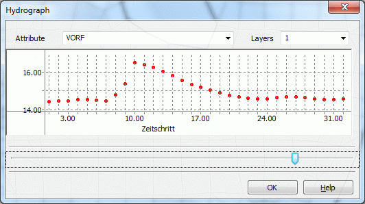
Transient data of deeper layers can also be selected.
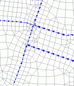
Water course systems 
After selecting this function, the existing water course systems are marked with arrows.
On water course systems…
By selecting this menu item it is possible to represent the attributes of the water course systems. These are the attributes:
VKST (Manning/Strickler coefficient, unit: m1/3/s)
VBRT (wetted perimeter, unit: m)
VGRD (bottom slope, unit: pro mille)
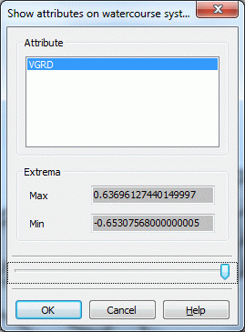
In particular, the assigned attributes of the water course systems can be checked with this menu item.
If the slope gradient (attribute VGRD) was calculated in the menu Special features Watercourse systems Attributes the slope direction on the element edges can be represented by arrows. Black arrows indicate a negative slope direction.
Texts at nodes/elements
Selecting this menu item, the texts at the nodes or elements specified in the mesh and/or 3d file are displayed.