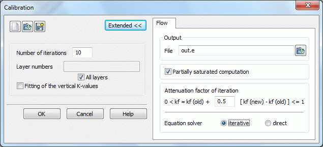
By activating the button "Extended" more parameters can be defined:

Output

The name of the output file is entered, default is the name out.e.

Fitting of the saturated thickness (2D) or partially saturated computation (3D)

For three-dimensional models, consideration of the saturated and unsaturated zones is possible (see also iteration of the free surface). The factors for the unsaturated elements are also computed using the previously calibrated data set. For two-dimensional models, the thickness can also be fitted, using the calibrated condition and the lower boundary of the aquifer, while respecting an eventually given maximum thickness. Fitting the thickness is only useful if the input thicknesses recorded during the model checking is different from the thickness of the saturated zone. Generally, this should not occur.

Attenuating the relative change of the K-value in an element (3D model only)

The changes in the K-values of an iteration to the next can be attenuated in various ways. This is recommended because the iteration oscillates slightly at a 'bad' initial state and K-values of adjacent elements can vary extremely.

A local attenuation of the relative change of the K-values considering the K-values of the adjacent elements is done automatically and was described above. For the simple attenuation of the changes of the K-value from an iteration to the next, the user can determine at this point an attenuation factor.

Instead of the computed new K-value k_n+1 (see iterative calibriation),

is applied with a default value of x = 0.5.

Equation solver

As solvers, the iterative PCG-solver or the direct Cholesky solvers are available. For meshes with more than 500 nodes, we recommend the iterative solver with respect to computing time and storage space. It does not compute an exact result, but the deviation will usually be negligible. The accuracy can be evaluated using the mass balance

Results of the calibration