Via Calculation  Inverse Calibration and selection of the calculation

appears the input window of the selected calculation module.
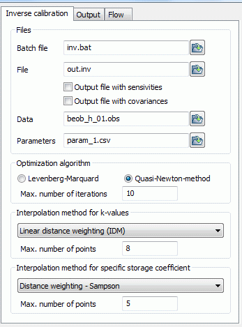
The description of the input parameters, especially those of the extended settings can be found in the chapters: "Input parameters" or "Extended Settings" of each calculation module. In addition to the parameters described there the inverse calibration requires more information. The dialog for entering the parameters for the inverse calibration is another notebook side in the extended settings (button "Extended"):

Files
An inverse calculation requires two batch files: The usual batch file with the parameters of the direct problem (sitra.bsi) and a batch file which contains the parameters of the inverse problem (default: inv.biv). The latter is defined here.
An inverse calculation creates two output files: The first output file contains the results of the latest direct calculation (out.s). Its name is defined in the main dialogue box. The second output file is named in this dialogue (default: out.inv). It contains the protocol of the inverse calculation with error tables for each iteration step, as well as the optimized parameters.
If the check boxes "output file with..." are enabled, the sensitivities (files param_name.sns, out.inv_tab.csv and out.inv.sens) and covariances (files kovarianz.csv) are written in additional output files.
The sensitivities provide a statement about how a change of the i.th parameter pi in the current set of parameters p affects the calculation result of the j. th observation date bj.
The covariance is a measure of the (linear) relationship between two random variables a and b with common distribution. The covariance is positive if a and b tend to having a linear relationship in the same direction, i.e. high values of a are associated with high values of b and low with low. On the other hand is the covariance negative, if a and b have a linear relationship in opposite directions, i.e. high values of a variable are associated with low values of the other variable. If the result is 0, then no linear relationship between the two variables a and b exists (non-linear relationships are possible) (from Wikipedia).
In the inverse modelling the covariances of the parameter values are calculated with respect to each other and written tabulated in the file kovarianz.csv.
The files containing the observation data and parameters are also specified here.
Optimization algorithm
Here you can select the optimization algorithm. Available are the Gauss-Newton algorithm based on Levenberg-Marquard and the Quasi-Newton algorithm.
The maximum number of iterations after which the optimization algorithm will be terminated regardless of the state of convergence has to be inserted.
Interpolation algorithm
This part defines the parameters for the interpolation of hydraulic conductivity or storage parameters within each zones (Z-KW or Z-SP), should such an interpolation be necessary. The available interpolation algorithms are:

Using the distance weighting, the definition of a maximum search radius is not required. This is in contrast to the module Interpolation. The interpolation always uses maximally the number of points with the smallest distance given in the data file.
