It is recommended to perform a calculation with 0 iterations first. So without much effort, the target function can be controlled. The results are written in the output file (here: out.inv). The shares for each parameter/measurement group are listed individually.
It is important to balance the shares of the target function. After the first inverse calculation (0 iterations), the shares of the target function are compared. The best-known sizes (usually the potential heads) should have the largest share of the target function (ZF).
Possible sources of errors:

K-values are weighted too heavily. This forbids the algorithm to calculate the K-values far away from the estimated value, so there are almost no changes in the K-values.

Quantities are weighted too heavily. Thus the measured potential heads lose their weight and the algorithm tries (in vain!) to bring the volumes to match. In most cases, the rule applies: If the potentials and the K-values fit, the amounts are also set in.

Transient hydrographs: The piezometer x is measured every day for over a year, in contrast, piezometer y is measured only once per month. When all measurements have the same  (i.e. equally weighted), the well x is weighted about 30 times stronger than y (365 measurements compared to 12 measurements).
 for well y
If the shares of the target function are balanced, the number of iterations is set to 10 and the inverse calculation is started again.
Output files

out.inv
 Import data/computational results
  iterated K-values.
Invpar.csv:

Invpar_xy.csv:

resan_pote.csv, resan_lkno.csv, resan_knot.csv (steady state only):

Example of the file resan_pote.csv

name.csv (transient only):

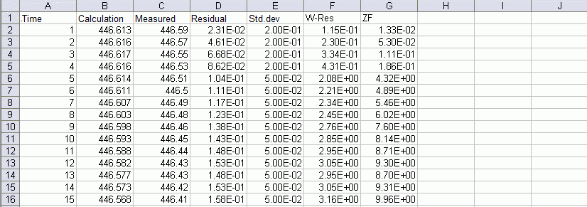
Example of a transient output file name.csv
