It is also possible to read structure data from "non-project" files (external format") into an existing project. These files do not have to be present in the *.str format. Different formats can be read in by clicking on Structure  Import ...
  .str, .txt, .csv, .arc, .shp. In the example, the structure data file s3_daten2.str was selected. (It was already downloaded from our homepage).
By saving the project (if desired, under a new name), the "old" and "new" structure data are written to the existing structure data file.
The new displayed structures are: Depth data of the lower edges of the model (UNTE), a MARK of the course of the stream and of the line-related leakage values of the course of the stream (LERA). Whereas the attributes MARK and LERA can be assigned directly as described in Direct assignment, the attribute UNTE must be interpolated in the present example element by element.
The entries for the individual interpolation methods are described in detail in chapter Calculation - Interpolation.
Via Attributes  Assign
  By interpolation, the following menu appears:
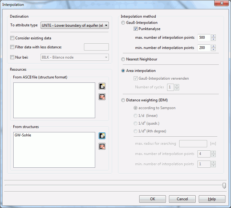
Interpolation of element data
When selecting Sources: "From structures" Add entry (button  ), another selection menu appears in which all existing structure data are listed. "UNTE" is selected. The results data type selected is also "UNTE". After pressing the OK button, the data will be interpolated and, after successful calculation, the following control window appears:
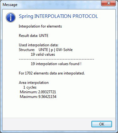
Interpolation protocol
The interpolation of the calibration potentials must be performed with particular care, since the calibration potentials are one of the most data types for calibrating the groundwater model. The groundwater measuring points in the area under investigation usually contain measured values at the time of calibration which have been saved to a file. Information regarding water levels of the main water course (POTE) and of the secondary water course system (VORF) is also known. These three data types are interpolated to give a calibration state which, after its first display, must be revised manually.
An example of a required revision are interpolated groundwater contour lines which show infiltration into groundwater where there is none. This situation is produced when the bed height of small secondary water course systems is set as the water course height, even though they are not carrying any water at all. In this case, the water course heights at the nodes for interpolation must be deleted.
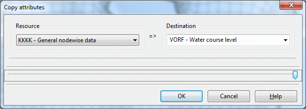
To include the attributes VORF and POTE (they were already assigned in the section Direct assignment), they are transferred from "VORF" or "POTE" to "EICH" via Attributes  Copy
Copy  Attribute-wise, in order to incorporate them in the interpolation as "existing data".
The menu for the interpolation of node data is available via Attributes  Assign
  By interpolation. There the file s3_gwmesspkte_neu.txt (download on our homepage!) is selected under Sources: "From ASCII file" Add entry. In addition, the menu item "Include existing data" is activated. This will include the already existing data under data type selected as results data (here EICH) in the interpolation points.
Here the results data are the calibration potentials (EICH). The data type and, for a 3D project, the layer number are defined under which the interpolated are data to be saved. The data type may differ from the codes of the structure data that may have been selected for interpolation!
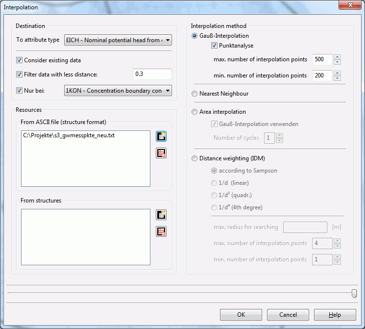
Interpolation of node data
Boundary conditions fo the interpolation:
By checking the check box "Filter data with less distance" interpolation points with nearby or identical coordinates can be excluded from the interpolation. The distance between all interpolation points for the minimum distance entered in the text box is checked. If two interpolation points have a smaller distance, the second interpolation point will not be used. First the existing data, then the structure data according to their sequence in the list and then the data from the ASCII files will be checked.
By selecting the check box only by node data can be interpolated in the area in which the selected data type is assigned.
Attention: In distance weighting, you have to ensure in the interpolation protocol that all FE nodes receive a value. If not, the "search radius" must be increased.
Moreover, the measured values and the position of the measuring points can be displayed at any time in the following input window by clicking on File  Import
  Overlay file
  *.txt.
First, the "Prev" button is clicked. At the bottom of the dialog then the columns are selected. In addition, a marker can be selected (type, height and colour).
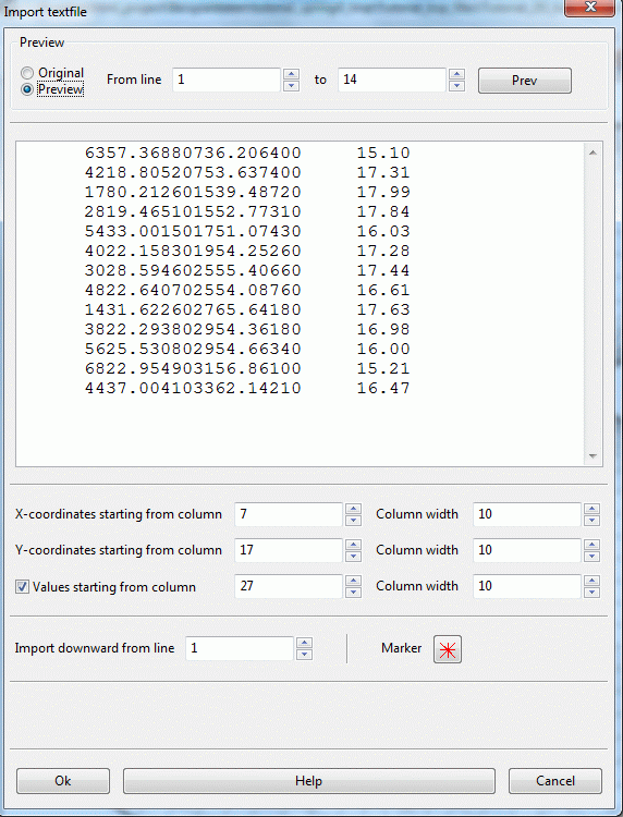
Importing a text file
After successful interpolation, the calibration potentials (EICH) can be displayed via View  Show attributes
  Isolines/Area plots/Values in the following form (Isolines in interval 12.50 to 20.0 and distance 0.5 m):
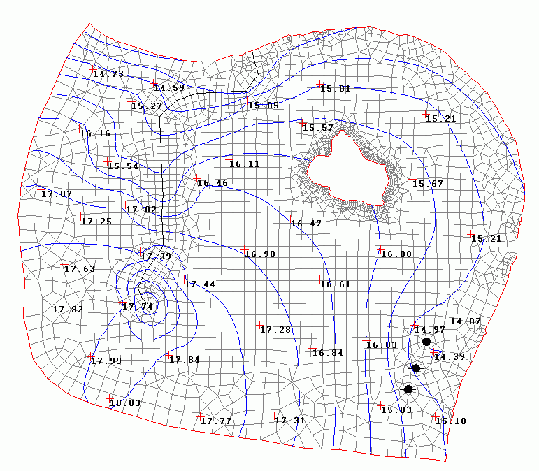
Interpolated initial potential heads, contour lines with a distance of 0.5 m
In the upper reach of the stream, the previously described, but not really present, groundwater infiltration of the stream can be seen, which is made visible by means of a "groundwater elevation". For calibration, the data were processed as follows: At 17 nodes of the upper reach of the water course system, the water course system potentials (VORF) are deleted, and the interpolation of the calibration potentials (EICH) described above is carried out again.
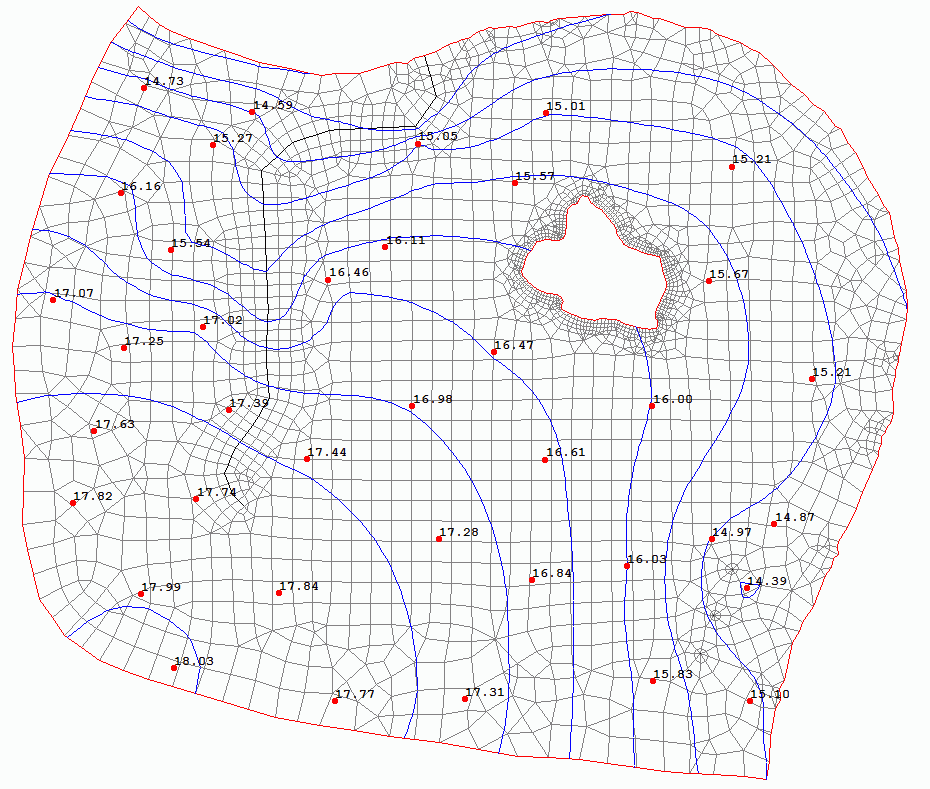
Interpolated initial potential heads considering the real groundwater situation
This is followed by reassigning the complete water course potentials (VORF) stored under an auxiliary attribute (e.g. KKKK).
Due to the low data density in the area of the pumping wells, their groundwater depletion is not reflected in the curve of the isolines.
Moreover, the ground level elevation must also be assigned. In most cases, ground level elevations are available as ASCII data records, which first have to be read into the structure data file: here “s3_gela.txt (zip)” (download on our homepage and unzip!).
The data are again assigned via Attributes  Assign
  By interpolation, Sources: From ASCII file: .txt.
The next step is a Manual attribute assignment 
