Further parameters can be defined by activating the "Advanced" button. The entries for the SITRA module are described first:

 

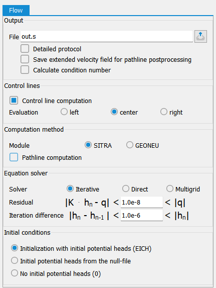
Output

The name of the output file is defined here. The default setting is the name out.s in the SITRA module or out.g in the GEONEU module.

In a detailed protocol (SITRA only), in addition to the intermediate times of a transient calculation, the mass balances (node by node) and any calculated volumes of control lines (node by node), calculated potential heads, concentrations or temperatures, saturations (for saturated/unsaturated calculation) and velocities are recorded.

 

Save extended velocity field for path line postprocessing

If this checkbox is activated, additional velocity vectors are saved during the steady state calculation with SITRA. In 2D, this takes place at the element edges and in the elements divided into sub-triangles. In 3D, the vectors are saved at the Gauss points of the elements.

After the flow calculation, the path lines button is then available in the menu under File Export... Path line output).

If the extended velocity field is saved, path line plots can be changed as required after a flow calculation (see Plotting Path lines).

 

Calculate condition number

If activated, the condition number of the matrix of the system of equations of the flow is calculated in each time step. It is a measure of the stability of the problem and the solution method and is defined as the ratio between the smallest and largest eigenvalues of the coefficient matrix. A low condition number indicates a well-posed system of equations with good convergence properties. A perfect system of equations has a condition number of 1.

 

Control line computation

(only if attribute KONT, p. 90) is present in the model file)

After activating the checkbox, the control lines are calculated. The evaluation is carried out either via the speed of the left or right adjacent element or by averaging the two velocities.

 

Computation method

The two computation modules SITRA and GEONEU are available. The default setting is a calculation with the SITRA module. If the path line calculation is activated at this point, the required data is also written to the background files. However, a subsequent change to the desired representation in the plot requires a new flow calculation.

 

Equation solver

Either the iterative PCG solver, the direct Cholesky equation solver (LU decomposition) or an algebraic multigrid equation solver can be selected as the equation solver. Due to its advantages in terms of computing time and memory space, the iterative equation solver is recommended for approximately 500 nodes and more. In contrast to the direct method, the solution is not calculated exactly, but the error is usually negligible. An accuracy check can be carried out using the mass balance specified in the output file. The multigrid equation solver is particularly recommended for models with large local differences in the hydraulic conductivity values.

• Iterative PCG solver: General CG method with preconditioning (Preconditioned Conjugate Gradient Solver) with block SSOR relaxation (Symmetric Successive Over Relaxation Method)

• Direct Cholesky equation solver: Gaussian elimination method

• Multigrid equation solver: CG method with preconditioning by multigrid method

 

Residual and iteration difference (iterative and multigrid solver only)

The basis of the iterative solution method is the boundary value problem defined as a variational problem, from which a quadratic function F(v) is obtained by discretisation, the minimum of which provides the required solution. Partial differentiation of F produces the familiar symmetrical and positive definite system of equations as a necessary condition for this minimisation:

K h* = q

With:

K = Hydraulic conductivity

h* = solution vector of potential heads

q = vector of sources/sinks

 

In the following, h* denotes the exact solution vector, which is now to be determined using an iterative procedure. With h as the so-called trial vector, the quadratic function can be written as follows:

 

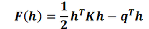
With:

h^T = transformed test vector of the potential heads

K = hydraulic conductivity matrix

h = trial vector of the potential heads

q^T = transformed vector of sources/sinks

 

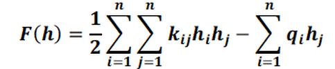
Or in index notation:

 

 

The partial differentiation according to hi provides:

 

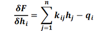
Here, δF / δh_i is the i-th component of the gradient or residual vector g for the test vector h,

 

 

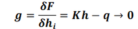
which is now run towards the value zero within the iterative process (or 1.0e-08 in this case according to the input for the residual).

The iteration process, which causes the residual vector g to approach zero, involves a systematic correction of a sequence of approximation vectors h in the following form:

 

h_i+1 = h_i + η_i d_{i ,} (i = 0, 1, 2, …)

 

In it, the trial vector h_i of the i-th iteration step is improved to the new approximation vector h_i+1 by means of the iteration vector d_i and a scalar step size η_i. The vector d_i indicates the direction of the relaxation pointing to the minimum of the function.

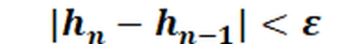
The iteration process is cancelled as soon as a previously set convergence limit/iteration difference ε is reached or exceeded, so that the accuracy of the result to be achieved is determined by the choice of this convergence measure/iteration difference ε.

The various vectors involved in determining the truncation barrier are then always related to each other by forming their Euclidean norm. This results in the following truncation criterion:

 

Calculation of outflow

The inputs for the discharge calculation are described in detail in the following chapter "Inputs for water system calculations".

 

Initial conditions

If the SITRA module is selected, the initial conditions for the steady state flow can also be defined. It is possible to take the initial potential heads from the attribute EICH or from the null-file, or the initial potential heads can be set = 0.

 

Input for water course system calculation