The discretisation of the area under investigation into individual, geometrically simple subregions (the finite elements which consist of triangles, quadrilaterals, prisms), is referred to as spatial discretisation. Within an element, the analysed variable (potential head, temperature, concentration) is approximated by the relevant equations. The reference points for the approximation of the function curve are the nodes. The nodes are located at the corners of the element, possibly on the element edges as well, and connect all neighbouring elements with each other, creating a coherent area.

The complex differential equation system, which describes the physical processes (flow and transport processes in porous media), is reduced to a discrete equation system for the solution of the test variables in the nodes by this approximation of the test variable curve at element level. The value of the analysed variable within an element can then be interpolated from the calculated node values.

The elements of the area are connected to each other via the nodes, which means that the approximated course of the analysed variable is also continuous across the element edges. To what extent the derivatives of the variables under investigation must be continuous depends on the physical problem. For flow and transport calculations in porous media, the continuity in the analysed variable is sufficient, which is why finite elements with linear approach functions are sufficiently accurate. When using linear approach functions, the nodes are located at the corners of the elements.

Approach functions, also known as shape functions, are functions that approximate the real function curve over the element as closely as possible when using the finite element method. The condition for this is the fulfilment of the continuity condition. As the nodal points are divided by at least two elements, the continuity condition is fulfilled when using the values at these points. The required function curve is approximately determined by interpolating the values at these nodal points. Shape functions are used to express the function curve u(x, y) through the node points. These have the property of always being 1 in the current node and 0 in the remaining nodes, so that u(x, y) is the sum of the number of nodes of u_i * N_i(x, y), where i is the number of the node in the element and u is the value at the node (derived from Wikipedia).

The linear shape function for the unit triangle with the coordinates of the three vertices (0,0), (1,0), (0,1) looks as follows (Fig. 50, linear approach): ):

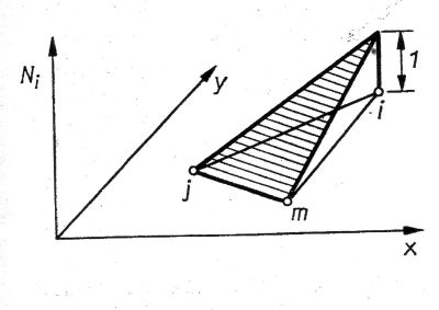
: Linear approach function for a triangle

A bilinear approach must be used for quadrilateral elements, as the edge of a quadrilateral element with a Z-coordinate not equal to 0 is not a straight line, but a curved line:

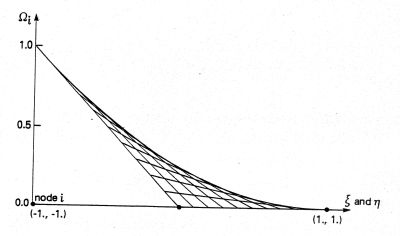
Bilinear approach function for a quadrilateral

Even more clearly is the shape function in the figure below:

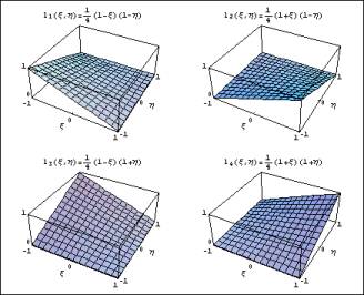
Bilinear approach for a quadrilateral element

Realisation in SPRING