Definition of Data Identifiers

To fully define the groundwater model, the nodes and elements of the FEM mesh are assigned attributes with a "four-letter" identifier. The underlying data types are described individually in the chapter "Data structure of the groundwater model” –Description of the data types.

 

In order to manage these attributes, it must be clear during model creation whether a data type is node- or element-related and whether special properties need to be taken into account (e.g. polygonal tension data or data that does not make sense for 3D models in the deeper layers, etc.). The meaning of the data type is not important at this stage.

For this reason, the initialisation of the data identifiers (in contrast to the model check) is not carried out permanently in the programme but is controlled via the xsusi.kenn file.

The file can be found at:

"C:\Users\Public\Documents\SPRING\Konfig" (Windows 7 or Windows Vista). This path varies depending on the operating system or hard drive partitioning (e.g. under Windows XP: "C:\Documents and Settings\All Users\Documents\SPRING\Konfig").

 

In addition to the general classification of the reference to nodes or elements, there is a distinction between:

• Simply assigned data: Each node or element can only be assigned one value per layer for this data type (example: a node in a layer can only have one fixed potential head (POTE attribute) and an element can only have one hydraulic conductivity value (KWER attribute) per layer). If such a data type is assigned twice to a node or element for any reason, you are asked whether the existing value (overwrite NONE) or the newly entered value (overwrite ALL) should be saved.

 

• Group data: Each node or element can receive several values per layer for this data type (example: a node can belong to several balance areas -BILA-).

 

• Polyline data (for node data): The data value is defined for a polyline of nodes, i.e. the order of the node numbers plays a decisive role in the data type (examples: LERA, MXKI, MXKE, ...).

 

• 2D or 3D data: There are data types for which it does not make sense to allow an assignment to deeper layers. These must be initialised as 2D data so that an assignment to layer numbers > 1 is not even possible. (Examples: GELA, MAEC, UNTE, UNDU, ...).

 

The identifiers are initialised as follows in the xsusi.kenn file:

 

First, the line beginning with ".KENNUNGEN." is searched for in the file. The following data is then read for each line until the end of the file or a line starting with ".END." is found:

 

 

 

Extract from an xsusi.kenn as an example for the attribute part:

 

.KENNUNGEN.

1KON k 3 Concentrations BC 1st type

ABRI k 3 Break-off height

AKON k 3 Initial concentrations

ASAT e 3 Initial saturation

BERG k 2 Subsidence

FLAE e 2 Surface infiltration (GW-Recharge)

GLEI ks3 Equal potential heads

KNOT k 3 Node inflows/outflows

KONT ks2 Control lines

UNTE e 2 Lower boundary of aquifer

VORF k 3 Watercourse stage

VERS e 2 Degree of sealing for recharge calculations

1DBR 1 Apperture (1D-Fractures)

1DMA 1 Thickness (1D- Fractures)

2DBR 2 Apperture (2D- Fractures)

.ENDE.

 

 

Unknown or user-defined identifiers

The user can also enter any identifiers in the structure file. In this case, the following input window appears when the project is opened with SPRING:

 

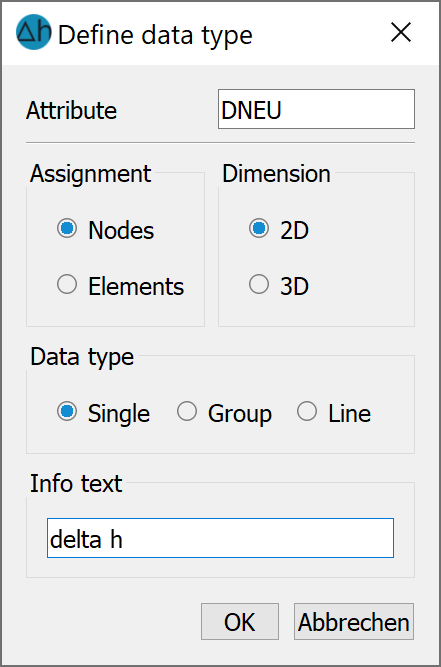
Here, the user can then define whether it should be a node- or element-related data type of the data type "Single", "Group" or "Line". If this new data type is to be permanent, it must be entered accordingly in the (user-specific) xsusi.kenn file.

 

Presetting the display parameters of the attributes

The xsusi.kenn file can be used to modify the default settings for the attribute display parameters (View Show attributes Attributes Isolines/area plots/values...). The default settings for the display of attributes are defined as follows, with a few exceptions:

• For single node data (e.g. terrain elevation or initial potential heads) 10 isolines at equidistant intervals

• For single element data (e.g. surface infiltration (FLAE) or hydraulic conductivity (KWER)) an area plot with 10 colour intervals (equidistant)

• For group data types (e.g. balance areas (BILA)) a circular plot with 10 equidistantly divided colour intervals

• For polyline data (e.g. leakage coefficient (LERA) or maximum infiltration at nodes (MXKI)) a representation of the polylines with a maximum of 10 colours (equidistant)

 

There are exceptions for a different default setting, e.g. for potential heads (POTE) or sources/sinks (KNOT). As these data types are simply assigned data, but are usually only defined locally at individual nodes, the default setting is a circular representation in the xsusi.kenn file.

In the xsusi.kenn file, the default settings for the display parameters of the attributes are initialised as follows:

After defining the attribute identifiers, the line starting with ".DARSTELLUNG." is searched for in the file. The display parameters are then read in the following form until the end of the file or a line starting with ".END." is found:

 

Line 1:

Column 1: * : stands for the initialisation character of a new identifier

Columns 2 - 5: KENN: stands for the four-letter identifier of the data type

Column 7: Layer number

 

Line 2:

Column 1:

k for circular representation

f for area representation

i for isoline representation

 

This is followed by the freely formatted number of the colour palette (for area or circle display) or the colour number for the isoline plot.

Then (unformatted) the height of the circle marker (for the largest value found) can be defined with r_max <= 6.0. If all circles are to be the same size, then r_max = 6.0 can be selected as the maximum radius.

 

Line 3:

These columns are without formatting. First there is a parameter for the choice of division: :

0: equidistant division

1: from/to/number

2: from/to/number (logarithmic)

3: from/to/distance

4: Individual values

 

For division types 0, 1 and 2, this is followed by the number of intervals and for division type 4 the number of individual values.

 

 

In the case of division line types 1 to 4, the following then follows:

Line 4:

For division types 1 and 2: Freely formatted 3 values: from, to, number

For division type 3: Freely formatted 3 values from, to, distance

For division type 4 with k or i: Freely formatted number of values for the isoline display or for the interval limits in the circular display (for 'k' interval limits)

For division type 4 with f: Freely formatted division of the intervals (minimum and maximum value for the interval limit in each case)

 

Extract from an xsusi.kenn as an example of the default display:

 

.DARSTELLUNG.

*AKON 1 /* Equal-value lines pen 5 */

i 5

0 10

*ASAT 1 /* Equal-value domains with palette 0 */

f 0

0 30

*BERG 1 /* Equal-value lines pen 5 */

i 5

0 10

*BILE 1 /* Equal-value domains with palette 0 */

f 0

0 10

*BILK 1 /* Circles with equal radius with palette 0 */

k 0 6.0

0 10

*DISP 1 /* Equal-value domains with palette 0 */

f 0

0 10

*EEEE 1 /* Equal-value domains with palette 0 */f 0

0 10.