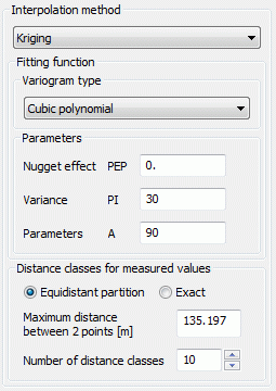
The most important step in an interpolation with the Kriging algorithm is to create a variogram. This shows the difference between two measured values versus the distance between the corresponding measuring points. The resulting statistical information is approximated by a variance function.

The first step creates a so-called experimental variogram. For that, distance classifications (distances in m) are defined:

with

 

 

Inside each class, a semivariance g_k(h) is computed from the measured values of all pairs of measuring points with the corresponding distance between:

with

 

where m_k represents the number of pairs (i, j) whose distance is part of the class K_k .

z_j denotes a point that has a distance h to the point z_i .

 

The user can define a maximum of 16 different distance classes. For each of them a table containing the significant variogram characteristics is output:

 

 

E. g. the table for an equidistant partition into 10 classes has the following appearance:

 

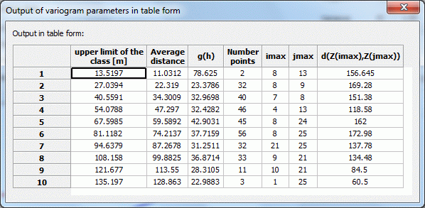
Tabular output of the variogram parameters

 

Additionally, to enable better comparison, the maximum distance between two data points is recorded.

The selected partition should guarantee that each class contains a minimum of one pair of data points. If possible, the number of pairs should have the same order of magnitude for all classes. If one pair of data points cannot be classified, the maximum distance of the last class is increased to the necessary value.

The experimental variogram shows the computed variances g_k(h) (column 4 of the table y-axis) versus the average distances h (column 3 of the table x-axis).

Limit of the x-axis is the calculated maximum distance between the measuring points to each other

Hence a function is to be found that best approximates this experimental variogram. This function is then used to compute the weighting factors λ_i(x, y) for the interpolation.

SPRING offers the following six types of functions as fitting functions:

Variogram h^A

Spherical variogram

Exponential variogram

Gaussian variogram

Cubic polynomial

Fitting polynomial

 

 

The types from (1) to (5) require the parameters PEP, PI and A:

PEP >= 0: so called 'nugget effect': Measure of the variability of the measured value (measurement error) g(0)=PEP

PI >= 0: Variance of the observed values

A >= 0: size of the region whose points are used for interpolation, for the types (2) to (5) the parameter A should be approximately the maximum distance

 

The following representation shows the meaning of each parameter schematically:

 

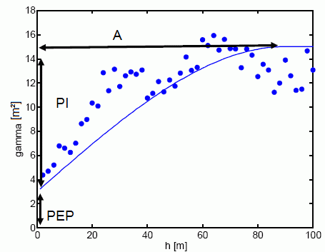
Schematic representation of the variogram parameters

 

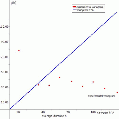
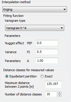
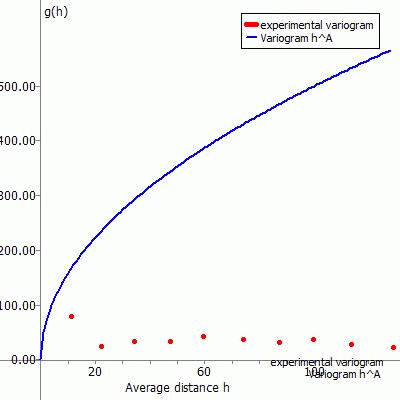
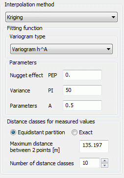
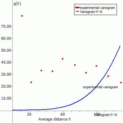
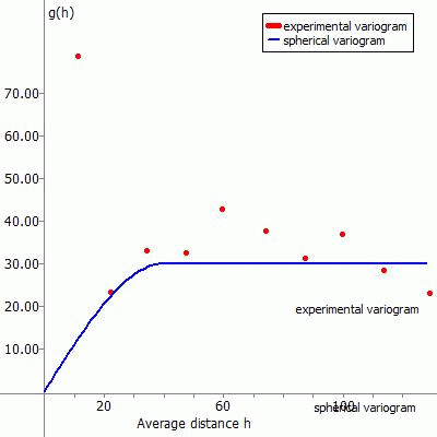
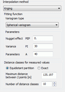
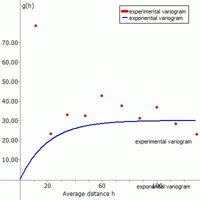
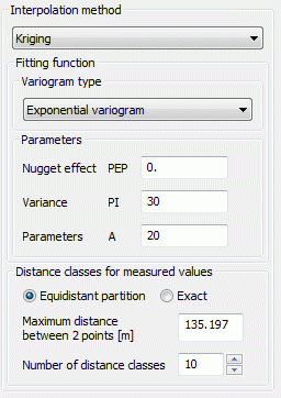
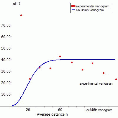
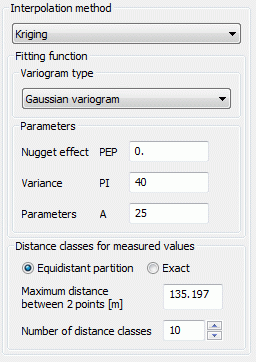
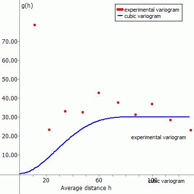
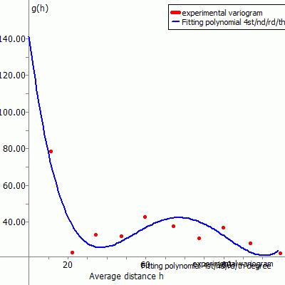
The following representations show the experimental variogram (red point) overlayed with the chosen function (blue) and the corresponding data input in SPRING for the different fitting functions.

 

(1) Variogram h^A:

The fitting function for this type of variogram is:

g(h) = PEP + PI * h^A

 

As a function of the parameter A there are three curves of the variogram possible:

 

Case 1: A = 1 (straight line)

 

 

Case 2: A < 1

 

 

Case 3: A > 1

 

 

 

(2) Spherical variogram:

The fitting function for this type of variogram is:

 

 

 

 

 

(3) Exponential variogram:

The fitting function for this type of variogram is:

 

 

 

 

(4) Gaussian variogram:

The fitting function for this type of variogram is:

g(h) = PEP + PI *( 1-exp (-H²)), with H = h/A

 

 

(5) Cubic polynomial:

The fitting function for this type of variogram is:

 

 

 

 

(6) Fitting polynomial form of a degree between 1 and 9

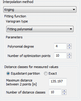
If the user selects type a fitting polynomial form, the degree of the polynomial (between 1 and 9) and the number of approximation points (for which the maximum is the number of classes) have to be defined.

The given example produces the following fitting polynomial form:

 

 

In general, the resulting functions should be increasing monotonously, and should approximate the given values as closely as possible. The quality of the variance function g(h) significantly influences the quality of the interpolated values using the Kriging procedure.

The creation of the variogram is the most important step, because of the high parameter sensitivity of the Kriging interpolation.

 

Kriging Interpolation