Minimization of the target function

The objective of inverse modelling is to minimize the target function. The target function consists of two main components:

ZF = ZF_obs+ ZF_par

Both the measured values (ZF_obs, i.e. potential heads, quantities) and the estimated values of the parameters (ZF_par, for example K-values, leakage coefficients, storage coefficients) enter into the target function. The shares are further divided

ZF_obs = ZF_POTE + ZF_LEAK + ZF_KNOT

ZF_par = ZF_KWER+ZF_LERA + ZF_KSPE

To determine the target function, a standard deviation is assigned to each parameter and measured value. This corresponds to the expected error of the parameter.

Each measurement value m, and each parameter value p is evaluated after each step of the inverse calibration as follows (method of type 'least squares’):

For the numerical solution of this nonlinear minimization problem, SPRING offers two different mathematical algorithms in the inverse modelling:

a Gauss-Newton-method by Levenberg-Marquard and

a gradient method by the Quasi-Newton-method

The shares of the target function of each measurement and of each parameter are summed. Chosing a small standard deviation results in a large proportion of the target function and thus in a high weighting. From a large standard deviation results a small proportion of the target function and thus a small weighting.

The following table shows the influence of weighting.

First, the two potentials H1 and H2 are listed. The residual is the same for both measurement points, however, a hundred-fold greater proportion of the target function results for H2, as this value is weighted with 10 cm standard deviation more strongly as H1 with 1 m standard deviation.

Another effect can be illustrated with the quantities Q1 and Q2. Depending on which unit is used a different weighting results by the same standard deviation. Therefore the standard deviations for quantities should always be in the range of 10-25% of the measurements (depending on accuracy).

Q1* and Q2* have a standard deviation of 10% - the shares of the target function are in the same order of magnitude.

As a final sample size is a parameter value (K-value) shown. Since this value is processed logarithmically, the standard deviation should be given in orders of magnitude from 0.1,…, 1.

		calculated	measured	Residual (calculated-measured)	Standard dev. (Sigma)	Proportion ZF (Residual²/sigma²)
1.	H1	65.285	66.040	-0.755	1	0.57
1.	H2	66.985	66.230	0.755	0.1	57.0
2.	Q1 [m³/d]	-10000	-5000	-5000	1	25000000
2.	Q2 [m³/d]	-0.116	-0.058	-0.058	1	0.0033
3.	Q1* [m³/d]	-10000	-5000	-5000	500	100
3.	Q2* [m³/d]	-0.116	-0.058	-0.058	0.006	93
4.	KWER [m/s]	1.5e-3	1.0e-03	Log(1.5e-3)-log(1.e-3)=-0.699	0.3	5.43

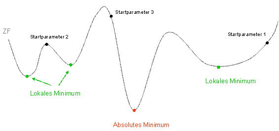
The following simplified illustration shows, why the initial values of the parameters can be crucial. The target function differs in size for different parameter values. There is an absolute minimum, as well as various local minima.

If you start the inverse modelling for example with the start parameter 1, the target function seeks to the associated local minimum. The target function for the start parameter 2 is on a local maximum and seeks to one of the two local minima.

The target function for the starting parameter 3 is at the highest, but the algorithm can reach the absolute minimum from this starting point. It is therefore quite reasonable to start the optimization process several times with different parameter values.

Formulation of the target function

Realization in SPRING