First, the existing (starting) K values are used to start an iteration run: Calculation  Model calibration. The following dialogue appears:
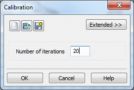
Calibration
After opening „Extended“ further settings can be made:
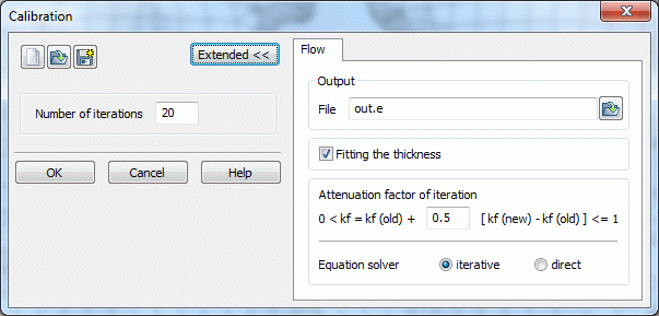
Extended parameters
After the calculation run, the isolines interpolated from the measured values are contrasted with the isolines obtained from the K values.
To do so, the model data type EICH and the resulting potentials are displayed after calibration (red) in the input window under File Plot generation "Top view/Map generation". Upon closing the module, the settings for this plot are saved to the batch file "plo.bpl" (predefined).
The following plot shows the result of the first calibration:
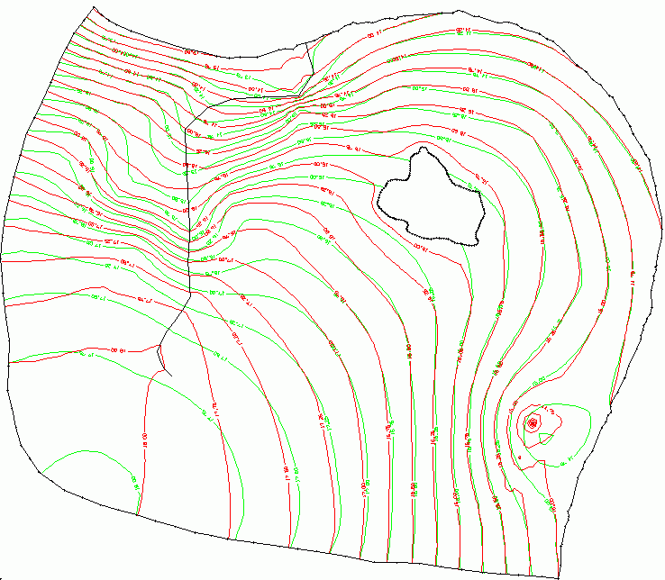
Calculated (red) and interpolated (green) potential heads after the 20th calibration
The next step is Generating a measured data difference plot and …