The following submenu appears:

 

 

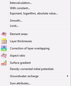
Intercalculation…

The following window appears:

 

 

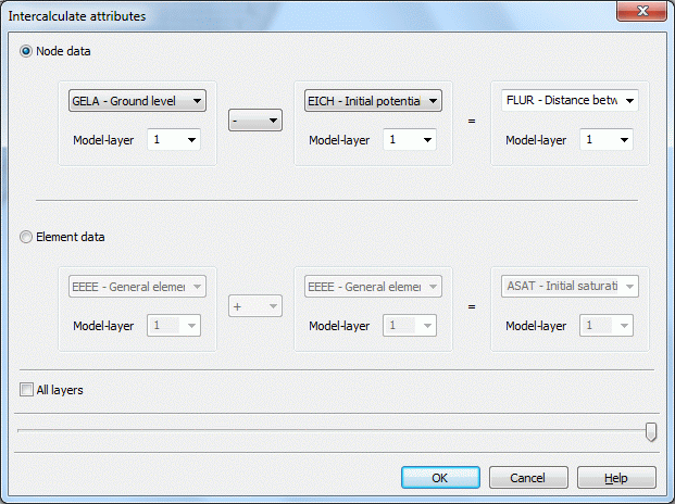
By using this function you can intercalculate two node wise or element wise data types and assign the result to a third node wise or element wise data type.

In case of a 3D model the data can be intercalculated either only in one layer or in all layers.

The resulting data type can be any identification even unknown to SPRING. Depending on the initial data types SPRING will save the new identification as node wise or element wise data type.

 

 

With constant…

The following window appears:

 

 

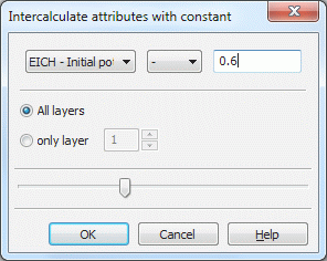
A selected node or element data type (for a 3D model in all or only one layer) can be calculated with a constant. As calculation method +, -, *, / and ^ are available. The result is assigned to the node/element instead ofthe former value. There is no further dialogue on substituting the original values by the calculation results.

 

 

Exponent, logarithm, absolute value…

In a 3D model the following window appears:

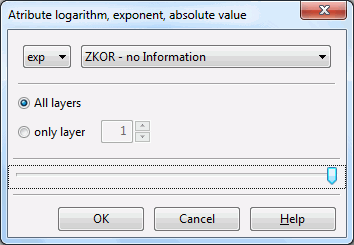
A 2D model lacks the input of a node or element layer.

By using this you can generate new data from your existing data with the help of the following functions:

 

In the case of a 3D model you can decide whether the values for all layers or the values for only one layer are intercalculated (transformed) by applying a logarithmic function. At each node or element (in all layers or only one layer) where a value x with the selected identifier exists it is transformed. The result is assigned to the node/element instead the former value. There is no further dialog on substituting the original values by the transformation results.

 

 

Smooth…

The following window appears for a 3D model:

 

 

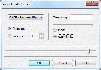
By using one this function you can smooth existing node wise or element wise data by mean value computation.

The new value for a node / element is obtained by adding the mean value of the adjacent nodes / elements to the original value:

 

 

Linear smoothing:

 

 

Logarithmic smoothing:

 

with:

w^neu:new value of a node or element

ω:weighting

w^alt:old value of the node or element

w_i:values of the adjacent nodes or elements

 

The larger you choose the weighting factor ω the smaller is the smoothing effect.

In case of a 3D model, you can choose whether the data should be smoothed in only one layer or in all layers, e.g. smooth KWER only in layer 7 or in all layers. Nevertheless, the smoothing algorithm uses only the horizontally adjacent element or node values, e.g. the values in layer k are smoothed depending only on values in the same layer k.

 

 

Limit…

The following window appears in a 3D model:

 

 

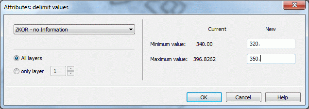
By using this function you can define upper and lower limits for existing data. In the case of 3D models, the values can be limited optionally in all layers or only in one layer.

 

After selecting the identifier and eventually the layer, the right part of the window reports the current minimum and maximum value. In the text boxes New the current extreme values can be substituted by new values. If you confirm the menu with OK the algorithm will compare all existing values with the new extreme values. The current value is substituted by either the new minimum or the new maximum for the case it is less or larger than allowed.

 

 

Element areas

By using this function the area XE "area:calculation" of all elements is calculated and stored in the modul file using the attribut AREA [m²].

 

Layer thicknesses (3D model only)

In case of a 3D model, the function Layer thickness computes the layer thickness XE "layer thickness:calculation" for all 3D layers by using the z-coordinates (ZKOR) in the following way:

 

ZMAE (layer n) = ZKOR (layer n) - ZKOR (layer n+1).

 

The layer thickness is stored as attribute ZMAE [m] in the model file.

 

 

Correction of layer overlapping (3D model only)

When an object (eg a deep pit) cuts through several layer XE "layer:overlapping" s, the nodes inside the object must be placed on the bottom (or top) layer affected. This is done using this function.

 

 

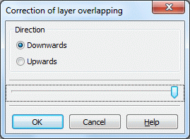
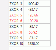
The incorrect layer boundaries are colored red in the node attributes dialog:

 

Aspect ratio

With this function the aspect ratio XE "aspect ratio:calculation" is calculated for all elements (of the top layer) with the momentary mesh geometry with the following rule:

Triangle elements: the aspect ratio corresponds the ratio between "inner circle" and "external circle" thus for an equilateral triangle the factor is 0.5.

Quadrangle elements: The aspect ratio corresponds the ratio between "minimal distance between the central point and the sides" and "maximum distance between central point and the sides" thus for a square the factor is 0.71.

It must point out that this is only a geometric quality criterion. For a flow calculation on the FE-mesh can other factors e.g. the direction of the flow control the evaluation of the element geometry.

The aspect ratio is stored as attribute FORM (single use, 2D-element data type) in the model file.

 

Surface gradient

With this function the surface gradient XE "surface gradient:calculation" is calculated for all elements. It is stored as attribute GGRD [%] in the model file.

 

 

Density-corrected initial potentials XE "Density-corrected initial potentials:density correction"

This menu item is only active if the attribute AKON is assigned in the model file (*.net or *.3d).

The potential heights h [m] EICH, POTE and VORF, entered in the model files or transient input file, must be converted in pressures p for the density-dependent flow calculation:

 

p = (h - z) * ρ * g

 

This is done with the density ρ = ρ₀ for the concentration c₀ = 0 or temperature T = T₀.

If the attributes 1KON or AKON are assigned to nodes with potential heights and hence the concentration c ≠ 0 (or T ≠ T₀ in the heat calculation), the potential heights must be converted with the density ρ = ρ(c) in a "corrected" water level. This is done with the following dialog:

 

 

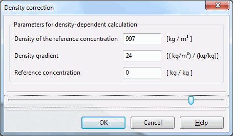
By entering the appropriate density parameters and confirm with OK, the potential heights are corrected and automatically stored in the model file. The parameters entered here correspond to the values that are entered in the dialog of the density-dependent mass transport.

 

 

Example:

The formula for the density-corrected potential height h_korr is:

 

h_korr = (h_Start - z) * ρ/ρ₀ + z

with:

h_korr [m] = with the density parameters corrected potential heights EICH, POTE, or VORF

h_Start [m] = POTE, EICH, or VORF at a node with a given 1KON or AKON

z [m] = height position of the node, in the 3D model is this the Z-coordinate, in the vertical model is this the Y-coordinate

ρ₀ [kg/m³] = density of the reference concentration c₀ = 0

ρ [kg/m³] = known/desired density ρ(c = c_max), c_max is usually the as 1KON or AKON entered maximum concentration

 

The in the dialog required density slope XE "density slope:calculation" α is obtained by changing the linear density function that is implemented in the program module SITRA:

 

ρ(c) = ρ₀ + α(c - c₀)

to:

α = (ρ(c_max) - ρ₀) / (c_max - c₀), if c = c_max is used.

 

Further information about the required parameters and conversions can be found in chapter "Density-dependent mass transport" .

 

 

Groundwater recharge

For the destination of the groundwater recharge XE "groundwater recharge:calculation" rate are three methods available in SPRING. These are the methods:

 

by Schroeder & Wyrwich with the following menu items:

 

 

by Meßer 2008 with the menu items:

 

 

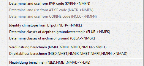
by soil water balance with the menu items:

 

 

If the basic attributes exist (KVNR, NATK or NCLC, NETP, FLUR, GELA), more attributes (NSFN, NMFN, NMKL, NMFK and NMGK are computed here. After that the parameters for the water balance equation (direct runoff NMAD and real evapotranspiration NMET) are to be calculated, so that at last the groundwater recharge rate can be destined.

A detailed description of the methods and the input data is given in chapter: „How To – Calculation of averaged groundwater recharge rates“ as well as on the website:

“Ein vereinfachtes Verfahren zur Berechnung der flächendifferenzierten Grundwasserneubildung in Mitteleuropa“.

 

 

RUBINFLUX

This menu item leads to the transient recharge computation with RUBINFLUX. A detailed description of the method and the input data is given in chapter: How To – “Calculating a transient groundwater recharge rate".

 

 

 

 

Sum attributes…

The following window appears in a 3D model:

 

 

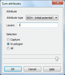
With this function attribute values are added up single, in an area or all and eventually for one or more layers. The result is shown in a dialogue box.

 

Menu item: Copy attributes