In a horizontal model the attribute GLEI (equal potential heads) is assigned to the nodes of a lake. If a lake is characterized like that, it is impossible to read the in- and outflow rates directly. First a flow (steady state or transient) calculation is done. Then you assign in SPRING the resulting potential heads to a user-defined attribute with Attributes Import model data/computation results... aaa result data: potential head e.g. KKKK. With Attributes Edit nodes and picking a boundary node of the lake, you get the calculated potential head of the lake.

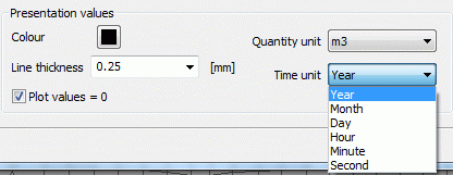
This value is assigned as attribute POTE to all boundary nodes of the lake, the attribute GLEI is deleted. At last the attribute BILK (integer value, identifies the balanced group) is assigned to these nodes to get the mass flow rates later on. After the flow computation you can read the mass flow rates of the boundary nodes in the output file. Or you display the resulting mass flow rate with the plot generation, where you can choose the quantity unit to be recalculated:

 

 

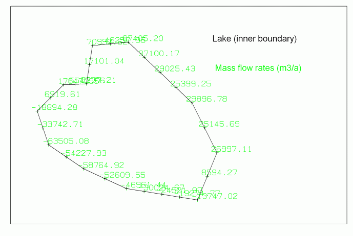
The unit m³/a is chosen. The following figure shows the lake with the calculated mass flow rates.

 

In- and outflow of a lake

 

The quantity of water flowing through the lake Q_in = Q_out is calculated by adding the negative and positive values. Depending on the discretization the values differ from each other in a marginal percentage:

 

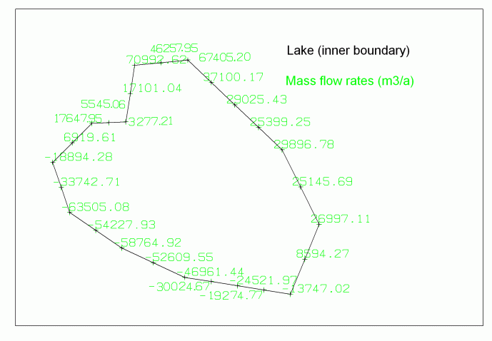
From adding the inflow (= negative sign it is an outflow of the model because of the inner boundary) results a mass flow rate of 430646 m³/a. From adding the outflow of the lake (= positive sign inflow into the model) results a mass flow rate of 422458 m³/a. The difference between the two rates amounts to - 8188 m³/a, which means a deviation of 0.5% of the water quantity flowing through the lake. A mesh refinement minimizes the deviation to -1032 m³/a respectively 0.2%, the water quantity flowing through the lake amounts to ca. 416790 m³/a.

 

 

In- and outflow of a lake after a mesh refinement